Row reduction (or Gaussian elimination) is the process of using row operations to reduce a matrix to row reduced echelon form. This procedure is used to solve systems of linear equations, invert matrices, compute determinants, and do many other things.
I'll begin by describing row operations, after which I'll show how they're used to do a row reduction.
Warning: Row reduction uses row operations. There are similar operations for columns which can be used in other situations (like computing determinants), but not here.
There are three kinds of row operations. (Actually, there is some redundancy here --- you can get away with two of them.) In the examples below, assume that we're using matrices with real entries (but see the notes under (b)).
(a) You may swap two rows.
Here is a swap of rows 2 and 3. I'll denote it by ![]() .
.
![$$\left[\matrix{ 1 & 2 & 3 \cr 4 & 5 & 6 \cr 7 & 8 & 9 \cr}\right] \quad\rightarrow\quad \left[\matrix{ 1 & 2 & 3 \cr 7 & 8 & 9 \cr 4 & 5 & 6 \cr}\right]\quad\halmos$$](row-reduction2.png)
(b) You may multiply (or divide) a row by a number that has a multiplicative inverse.
If your number system is a field, a number has a multiplicative inverse if and only if it's nonzero. This is the case for most of our work in linear algebra.
If your number system is more general (e.g. a commutative ring with identity), it requires more care to ensure that a number has a multiplicative inverse.
Here is row 2 multiplied by ![]() . I'll denote this operation by
. I'll denote this operation by
![]() .
.
![$$\left[\matrix{ 1 & 2 & 3 \cr 4 & 5 & 6 \cr 7 & 8 & 9 \cr}\right] \quad\rightarrow\quad \left[\matrix{ 1 & 2 & 3 \cr 4 \pi & 5 \pi & 6 \pi \cr 7 & 8 & 9 \cr}\right]\quad\halmos$$](row-reduction5.png)
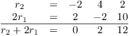
(c) You may add a multiple of a row to another row.
For example, I'll add 2 times row 1 to row 2. Notation: ![]() .
.
![$$\left[\matrix{ 1 & -1 & 5 \cr -2 & 4 & 2 \cr 1 & 3 & 1 \cr}\right] \quad\rightarrow\quad \left[\matrix{ 1 & -1 & 5 \cr 0 & 2 & 12 \cr 1 & 3 & 1 \cr}\right]$$](row-reduction7.png)
Notice in "![]() " row 2 is the
row that changes; row 1 is unchanged. You figure the "
" row 2 is the
row that changes; row 1 is unchanged. You figure the "![]() " on scratch paper, but you don't actually
change row 1.
" on scratch paper, but you don't actually
change row 1.
You can do the arithmetic for these operations in your head, but use scratch paper if you need to. Here's the arithmetic for the last operation:
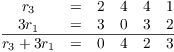
Since the "multiple" can be negative, you may also subtract a multiple of a row from another row.
For example, I'll subtract 4 times row 1 from row 2. Notation: ![]() .
.
![$$\left[\matrix{ 1 & 2 & 3 \cr 4 & 5 & 6 \cr 7 & 8 & 9 \cr}\right] \quad\rightarrow\quad \left[\matrix{ 1 & 2 & 3 \cr 0 & -3 & -6 \cr 7 & 8 & 9 \cr}\right]$$](row-reduction12.png)
Notice that row 1 was not affected by this operation.
Likewise, if you do ![]() , row 17 changes and row 31 does not.
, row 17 changes and row 31 does not.
Operation (c) is probably the one that you will use the most.
You may wonder: Why are these operations allowed, but not others? We'll see that these row operations imitate operations we can perform when we're solving a system of linear equations.
Example. In each case, tell whether the operation is a valid single row operation on a matrix with real numbers. If it is, say what it does (in words).
(a) ![]() .
.
(b) ![]() .
.
(c) ![]() .
.
(d) ![]() .
.
(e) ![]() and
and ![]() .
.
(a) This operation swaps row 5 and row 3.![]()
(b) This isn't a valid row operation. You can't add or subtract a
number from the elements in a row.![]()
(c) This adds ![]() times row 17 to row 3 (and replaces row 3
with the result). Row 17 is not changed.
times row 17 to row 3 (and replaces row 3
with the result). Row 17 is not changed.![]()
(d) This isn't a valid row operation, though you could accomplish it
using two row operations: First, multiply row 6 by 5; next,
add 11 times row 2 to the new row 6.![]()
(e) This is not a valid row operation. It's actually two row
operations, not one. The only row operation that changes two rows at
once is swapping two rows.![]()
Matrices can be used to represent systems of linear equations. Row operations are intended to mimic the algebraic operations you use to solve a system. Row-reduced echelon form corresponds to the "solved form" of a system.
A matrix is in row reduced echelon form if the following conditions are satisfied:
(a) The first nonzero element in each row (if any) is a "1" (a leading entry).
(b) Each leading entry is the only nonzero element in its column.
(c) All the all-zero rows (if any) are at the bottom of the matrix.
(d) The leading entries form a "stairstep pattern" from northwest to southeast:
![$$\left[\matrix{ 0 & 1 & 6 & 0 & 0 & 2 & \ldots \cr 0 & 0 & 0 & 1 & 0 & -1 & \ldots \cr 0 & 0 & 0 & 0 & 1 & 4 & \ldots \cr 0 & 0 & 0 & 0 & 0 & 0 & \ldots \cr \vdots & \vdots & \vdots & \vdots & \vdots & \vdots & \cr}\right]$$](row-reduction21.png)
In this matrix, the leading entries are in positions ![]() ,
, ![]() ,
, ![]() , ... .
, ... .
Here are some matrices in row reduced echelon form. This is the ![]() identity matrix:
identity matrix:
![$$\left[\matrix{ 1 & 0 & 0 \cr 0 & 1 & 0 \cr 0 & 0 & 1 \cr}\right]$$](row-reduction26.png)
The leading entries are in the ![]() ,
, ![]() , and
, and ![]() positions.
positions.
This matrix is in row reduced echelon form; its leading entries are
in the ![]() and
and ![]() positions.
positions.
![$$\left[\matrix{ 1 & 5 & 0 & 2 \cr 0 & 0 & 1 & 3 \cr 0 & 0 & 0 & 0 \cr}\right]$$](row-reduction32.png)
A leading entry must be the only nonzero number in its column. In
this case, the "5" in the ![]() position does not
violate the definition, because it is not in the same column as a
leading entry. Likewise for the "2" and "3" in
the fourth column.
position does not
violate the definition, because it is not in the same column as a
leading entry. Likewise for the "2" and "3" in
the fourth column.
This matrix has more rows than columns. It is in row reduced echelon form.
![$$\left[\matrix{1 & 0 \cr 0 & 1 \cr 0 & 0 \cr 0 & 0 \cr}\right]$$](row-reduction34.png)
This row reduced echelon matrix has leading entries in the ![]() ,
, ![]() , and
, and ![]() positions.
positions.
![$$\left[\matrix{ 1 & 0 & 6 & 0 & 2 \cr 0 & 1 & 1 & 0 & -3 \cr 0 & 0 & 0 & 1 & 4 \cr 0 & 0 & 0 & 0 & 0 \cr}\right]$$](row-reduction38.png)
The nonzero numbers in the third and fifth columns don't violate the definition, because they aren't in the same column as a leading entry.
A zero matrix is in row-reduced echelon form, though it won't normally come up during a row reduction.
![$$\left[\matrix{ 0 & 0 & 0 & 0 \cr 0 & 0 & 0 & 0 \cr 0 & 0 & 0 & 0 \cr}\right]$$](row-reduction39.png)
Note that conditions (a), (b), and (d) of the definition are vacuously satisfied, since there are no leading entries.
Just as you may have wondered why only certain operations are allowed as row operations, you might wonder what row reduced echelon form is for. "Why do we want a matrix to look this way?" As with the question about row operations, the rationale for row reduced echelon form involves solving systems of linear equations. If you want, you can jump ahead to the section on solving systems of linear equations and see how these questions are answered. In the rest of this section, I'll focus on the process on row reducing a matrix and leave the reasons for later.
Example. The following real number matrices are not in row reduced echelon form. In each case, explain why.
(a) ![$\displaystyle
\left[\matrix{1 & 0 & 0 \cr 0 & 7 & 0 \cr 0 & 0 & 1 \cr}\right]$](row-reduction40.png)
(b) ![$\displaystyle
\left[\matrix{1 & 0 & -3 \cr 0 & 1 & 5 \cr 0 & 0 & 1 \cr}\right]$](row-reduction41.png) .
.
(c) ![$\displaystyle
\left[\matrix{0 & 0 & 0 & 0 \cr 0 & 1 & 0 & -1 \cr 0 & 0 & 1 & 9
\cr}\right]$](row-reduction42.png) .
.
(d) ![$\displaystyle
\left[\matrix{1 & 37 & 2 & -1 \cr 0 & 1 & -3 & 0 \cr 0 & 0 & 0 & 0
\cr}\right]$](row-reduction43.png) .
.
(e) ![$\displaystyle
\left[\matrix{0 & 1 & 7 & 10 \cr 1 & 0 & 4 & -5 \cr 0 & 0 & 0 & 0
\cr}\right]$](row-reduction44.png) .
.
(a) The first nonzero element in row 2 is a "7", rather
than a "1".![]()
(b) The leading entry in row 3 is not the only nonzero element in its
column.![]()
(c) There is an all-zero row above a nonzero row.![]()
(d) The leading entry in row 2 is not the only nonzero element in its
column.![]()
(e) The leading entries do not form a "stairstep pattern"
from northwest to southeast.![]()
Row reduction is the process of using row
operations to transform a matrix into a row reduced echelon matrix.
As the algorithm proceeds, you move in stairstep fashion from
"northwest" to "southeast" through different
positions in the matrix. In the description below, when I say that
the current position is ![]() , I mean that your current location is in row i and
column j. The current position refers to a
location, not the element at that location (which I'll
sometimes call the current element or current entry). The current
row means the row of the matrix containing the current position
and the current column means the column of the
matrix containing the current position.
, I mean that your current location is in row i and
column j. The current position refers to a
location, not the element at that location (which I'll
sometimes call the current element or current entry). The current
row means the row of the matrix containing the current position
and the current column means the column of the
matrix containing the current position.
Some notes:
1. There are many ways to arrange the algorithm. For instance,
another approach gives the ![]() -decomposition of a matrix.
-decomposition of a matrix.
2. Trying to learn to row reduce by following the steps below is pretty tedious, and most people will want to learn by doing examples. The steps are there so that, as you're learning to do this, you have some idea of what to do if you get stuck. Skim the steps first, then move on to the examples; go back to the steps if you get stuck.
3. As you gain experience, you may notice shortcuts you can take which don't follow the steps below. But you can get very confused if you focus on shortcuts before you've really absorbed the sense of the algorithm. I think it's better to learn to use a correct algorithm "by the book" first, the test being whether you can reliably and accurately row reduce a matrix. Then you can consider using shortcuts.
4. The algorithm is set up so that if you stop in the middle of a row reduction --- maybe you want to take a break to have lunch --- and forget where you were, you can restart the algorithm from the very start. The algorithm will quickly take you through the steps you already did without redoing the computations and leave you where you left off.
5. There's no point in doing row reductions by hand forever, and for larger matrices (as would occur in real world applications) it's impractical. At some point, you'll use a computer. However, I think it's important to do enough examples by hand that you understand the algorithm.
Algorithm: Row Reducing a Matrix
We'll assume that we're using a number system which is a field. Remember that this means that every nonzero number has a multiplicative inverse --- or equivalently, that you can divide by any nonzero number.
Step 1. Start with the current position at
![]() .
.
Step 2. Test the element at the current position. If it's nonzero, go to Step 2(a); if it's 0, go to Step 2(b).
Step 2(a). If the element at the current position is nonzero, then:
(i) Divide all the elements in the current row by the current element. This makes the current element 1.
(ii) Add or subtract multiples of the current row from the other rows in the matrix so that all the elements in the current column (except for the current element) are 0.
(iii) Move the current position to the next row and the next column --- that is, move one step down and one step to the right. If doing either of these things would take you out of the matrix, then stop: The matrix is in row-reduced echelon form. Otherwise, return to the beginning of Step 2.
Step 2(b). If the element at the current position is 0, then look at the elements in the current column below the current element. There are two possibilities.
(i) If all the elements below the current element are 0, then move the current position to the next column (in the same row) --- that is, move one step right. If doing this would take you out of the matrix, then stop: The matrix is in row-reduced echelon form. Otherwise, return to the beginning of Step 2.
(ii) If some element below the current element is nonzero, then swap the current row and the row containing the nonzero element. Then return to the beginning of Step 2.
Example. For each of the following real number
matrices, assume that the current position is ![]() . What is the next step in the row-reduction
algorithm?
. What is the next step in the row-reduction
algorithm?
(a)
![$$\left[\matrix{ \lower3.5pt\boxit{\hbox{2}} & -4 & 0 & 8 \cr 3 & 0 & 0 & 1 \cr -1 & 0 & 1 & 1 \cr}\right]$$](row-reduction49.png)
(b)
![$$\left[\matrix{ \lower3.5pt\boxit{\hbox{1}} & -2 & 0 & 4 \cr 3 & 0 & 0 & 1 \cr -1 & 0 & 1 & 1 \cr}\right]$$](row-reduction50.png)
(c)
![$$\left[\matrix{ \lower3.5pt\boxit{\hbox{1}} & -2 & 0 & 4 \cr 0 & 6 & 0 & -11 \cr 0 & -2 & 1 & 5 \cr}\right]$$](row-reduction51.png)
(d)
![$$\left[\matrix{ \lower3.5pt\boxit{\hbox{0}} & 2 & 1 & -1 \cr 0 & 8 & -11 & 4 \cr 7 & 5 & 0 & -2 \cr}\right]$$](row-reduction52.png)
(e)
![$$\left[\matrix{ \lower3.5pt\boxit{\hbox{0}} & 1 & 0 & 3 \cr 0 & 1 & 5 & 17 \cr 0 & 2 & -3 & 0 \cr}\right]$$](row-reduction53.png)
(a) The element in the current position is 2, which is nonzero. So I divide the first row by 2 to make the element 1:
![$$\left[\matrix{ 2 & -4 & 0 & 8 \cr 3 & 0 & 0 & 1 \cr -1 & 0 & 1 & 1 \cr}\right] \matrix{\rightarrow \cr r_1 \to \frac{1}{2} r_1 \cr} \left[\matrix{ 1 & -2 & 0 & 4 \cr 3 & 0 & 0 & 1 \cr -1 & 0 & 1 & 1 \cr}\right]\quad\halmos$$](row-reduction54.png)
(b) The element in the current position is 1. There are nonzero elements below it in the first column, and I want to turn those into zeros. To turn the 3 in row 2, column 1 into a 0, I need to subtract 3 times row 1 from row 2:
![$$\left[\matrix{ \lower3.5pt\boxit{\hbox{1}} & -2 & 0 & 4 \cr 3 & 0 & 0 & 1 \cr -1 & 0 & 1 & 1 \cr}\right] \matrix{\rightarrow \cr r_2 \to r_2 - 3 r_1 \cr} \left[\matrix{ 1 & -2 & 0 & 4 \cr 0 & 6 & 0 & -11 \cr -1 & 0 & 1 & 1 \cr}\right]\quad\halmos$$](row-reduction55.png)
(c) The element in the current position is 1, and it's the only nonzero element in its column. So I move the current position down one row and to the right one column. No row operation is performed, and the matrix doesn't change.
![$$\left[\matrix{ \lower3.5pt\boxit{\hbox{1}} & -2 & 0 & 4 \cr 0 & 6 & 0 & -11 \cr 0 & -2 & 1 & 5 \cr}\right] \quad\hbox{to}\quad \left[\matrix{ 1 & -2 & 0 & 4 \cr 0 & \lower3.5pt\boxit{\hbox{6}} & 0 & -11 \cr 0 & -2 & 1 & 5 \cr}\right]\quad\halmos$$](row-reduction56.png)
(d) The element in the current position is 0. I look below it and see a nonzero element in the same column in row 3. So I swap row 1 and row 3; the current position remains the same, and I return to the start of Step 2.
![$$\left[\matrix{ \lower3.5pt\boxit{\hbox{0}} & 2 & 1 & -1 \cr 0 & 8 & -11 & 4 \cr 7 & 5 & 0 & -2 \cr}\right] \matrix{\rightarrow \cr r_1 \leftrightarrow r_3 \cr} \left[\matrix{ \lower3.5pt\boxit{\hbox{7}} & 5 & 0 & -2 \cr 0 & 8 & -11 & 4 \cr 0 & 2 & 1 & -1 \cr}\right]\quad\halmos$$](row-reduction57.png)
(e) The element in the current position is 0. There are no nonzero elements below it in the same column. I don't perform any row operations; I just move the current position to the next column (in the same row). The matrix does not change.
![$$\left[\matrix{ \lower3.5pt\boxit{\hbox{0}} & 1 & 0 & 3 \cr 0 & 1 & 5 & 17 \cr 0 & 2 & -3 & 0 \cr}\right] \quad\hbox{to}\quad \left[\matrix{ 0 & \lower3.5pt\boxit{\hbox{1}} & 0 & 3 \cr 0 & 1 & 5 & 17 \cr 0 & 2 & -3 & 0 \cr}\right]\quad\halmos$$](row-reduction58.png)
There are two questions which arise with this algorithm:
1. Why does the algorithm terminate? (Could you ever get stuck and never finish?)
2. When the algorithm does terminate, why is the final matrix in row-reduced echelon form?
The first question is easy to answer. As you execute the algorithm, the current position moves through the matrix in "stairstep" fashion:
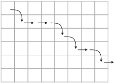
The cases in Step 2 cover all the possibilities, and in each case, you perform a finite number of row operations (no larger than the number of rows in the matrix, plus one) before you move the current position. Since you're always moving the current position to the right (Step 2(b)(i)) or to the right and down (Step 2(a)(iii)), and since the matrix has only finitely many rows and columns, you must eventually reach the edge of the matrix and the algorithm will terminate.
As for the second question, I'll give a very informal argument using the matrix with the "stairstep" path pictured above.
First, if you moved the current position down and to the right, the previous current element was a 1, and every other element in its column must be 0. In the matrix with the "stairstep" path I gave above, this means that each spot where a curved arrow starts must be a 1, and all the other elements in the column with a 1 must be 0. Hence, the matrix must look like this:
![$$\left[\matrix{ 1 & * & * & 0 & 0 & * & 0 & * \cr 0 & * & * & 1 & 0 & * & 0 & * \cr 0 & * & * & 0 & 1 & * & 0 & * \cr 0 & * & * & 0 & 0 & * & 1 & * \cr 0 & * & * & 0 & 0 & * & 0 & * \cr 0 & * & * & 0 & 0 & * & 0 & * \cr}\right]$$](row-reduction60.png)
(The *'s stand for elements which I don't know.)
Next, notice that if you moved the current position to the right (but not down), then the previous current element and everything below it must have been 0. In terms of the picture, every spot where a right arrow starts must be a 0, and all the elements below it must be 0. Now I know that the matrix looks like this:
![$$\left[\matrix{ 1 & * & * & 0 & 0 & * & 0 & * \cr 0 & 0 & 0 & 1 & 0 & * & 0 & * \cr 0 & 0 & 0 & 0 & 1 & * & 0 & * \cr 0 & 0 & 0 & 0 & 0 & 0 & 1 & * \cr 0 & 0 & 0 & 0 & 0 & 0 & 0 & 0 \cr 0 & 0 & 0 & 0 & 0 & 0 & 0 & 0 \cr}\right]$$](row-reduction61.png)
In either case, you don't move your current position until the column you're in is "fixed" --- that is, your column and everything to the left of it is in row reduced echelon form. When the algorithm terminates, the whole matrix is in row reduced echelon form.
Notice that this matrix is in row-reduced echelon form.
Row reduction is a key algorithm in linear algebra, and you should work through enough examples so that you understand how it works. So here we go with some full examples --- try to do as much of the work by yourself as possible. I will start by giving lots of details, but gradually give fewer so that this doesn't become too long and tedious.
Example. Row reduce the following matrix over
![]() to row-reduced echelon form.
to row-reduced echelon form.
![$$\left[\matrix{ 0 & 0 & 1 & -1 & -2 \cr 2 & -4 & -2 & 4 & 18 \cr -1 & 2 & 3 & -5 & -16 \cr}\right]$$](row-reduction63.png)
I will follow the steps in the algorithm I described earlier. Since this is our first example, I'll explain the steps and the reasons for them in a lot of detail. This will make the solution a bit long!
We start out in the upper-left hand corner (row 1, column 1), where the entry is 0. According to the algorithm, I look below that entry to see if I can find a nonzero entry in the same column. The entry in row 2, column 1 is 2, which is nonzero. So I swap row 1 and row 2:
![$$\left[\matrix{ 0 & 0 & 1 & -1 & -2 \cr 2 & -4 & -2 & 4 & 18 \cr -1 & 2 & 3 & -5 & -16 \cr}\right] \matrix{\to \cr r_{1} \leftrightarrow r_{2} \cr} \left[\matrix{ 2 & -4 & -2 & 4 & 18 \cr 0 & 0 & 1 & -1 & -2 \cr -1 & 2 & 3 & -5 & -16 \cr}\right]$$](row-reduction64.png)
Note that the current position hasn't changed: It is still row 1, column 1. But the entry there is now 2, which is nonzero. The algorithm says that if the entry is nonzero but not equal to 1, then divide the row by the entry. So I divide row 1 by 2:
![$$\left[\matrix{ 2 & -4 & -2 & 4 & 18 \cr 0 & 0 & 1 & -1 & -2 \cr -1 & 2 & 3 & -5 & -16 \cr}\right] \matrix{\to \cr r_{1} \to \dfrac{1}{2} r_{1} \cr} \left[\matrix{ 1 & -2 & -1 & 2 & 9 \cr 0 & 0 & 1 & -1 & -2 \cr -1 & 2 & 3 & -5 & -16 \cr}\right]$$](row-reduction65.png)
Now the element in the current position is 1 --- it is what I want for the leading entry in each row.
The algorithm then tells me to look below and above the current entry in its column. Wherever I see a nonzero entry above or below, I add or subtract a multiple of the row to make the nonzero entry 0. Most of the row operations you do will be operations of this kind.
There are no entries above the 1 is row 1, column 1. Below it there is 0 in row 2 and -1 in row 3. The 0 in row 2 is already what I want. So I just have to fix the -1 in row 3. What multiple of 1 do you add to -1 to get 0? Obviously, you just add (the "multiple" is 1). So I add row 1 to row 3:
![$$\left[\matrix{ 1 & -2 & -1 & 2 & 9 \cr 0 & 0 & 1 & -1 & -2 \cr -1 & 2 & 3 & -5 & -16 \cr}\right] \matrix{\to \cr r_{3} \to r_{3} + r_{1} \cr} \left[\matrix{ 1 & -2 & -1 & 2 & 9 \cr 0 & 0 & 1 & -1 & -2 \cr 0 & 0 & 2 & -3 & -7 \cr}\right]$$](row-reduction66.png)
Notice that row 3 changed but row 1 did not.
Let's look at where we are. The current position is still row 1, column 1. The first column is "fixed", in the sense that it's as it should be for row-reduced echelon form. So we move on, and the algorithm tells me to move the current position one step down and one step to the right. That puts the current position at row 2, column 2.
The element in row 2, column 2 is 0. So I'm in the situation I was in at the very start. I look below this element in column 2 and try to find a nonzero element --- but there is none. The element in row 3, column 2 is also 0. Note: I don't look at the -2 in row 1, column 2 --- I can only look below the current entry if it is 0.
So I can't do a row swap as I did earlier. The algorithm tells me that, in this case, I should just move the current position one step to the right. Now it is row 2, column 3, and the current entry is 1.
Since the current entry is 1, I don't need to divide row 2 by anything. I look below and above the current entry; I see 2 below and -1 above. So I add or subtract multiple of row 2 to or from row 3 and row 1 to make the 2 and -1 into 0.
First, I'll add row 2 to row 1 to make the -1 into 0. Next, I'll subtract 2 times row 2 from row 3 to make the 2 into 0.
![$$\left[\matrix{ 1 & -2 & -1 & 2 & 9 \cr 0 & 0 & 1 & -1 & -2 \cr 0 & 0 & 2 & -3 & -7 \cr}\right] \matrix{\to \cr r_{1} \to r_{1} + r_{2} \cr} \left[\matrix{ 1 & -2 & 0 & 1 & 7 \cr 0 & 0 & 1 & -1 & -2 \cr 0 & 0 & 2 & -3 & -7 \cr}\right] \matrix{\to \cr r_{3} \to r_{3} - 2 r_{2} \cr} \left[\matrix{ 1 & -2 & 0 & 1 & 7 \cr 0 & 0 & 1 & -1 & -2 \cr 0 & 0 & 0 & -1 & -3 \cr}\right]$$](row-reduction67.png)
You can do these in either order.
If you're worried about the -2 in row 1, column 2, you don't need to worry. It is not a problem because it is not in the same column as a leading entry (the 1s in row 1, column 1 and row 2, colum n 3).
Column 3 is now done. The algorithm tells me to move down one step and right one step. This puts the current position at row 3, column 4. The entry there is -1. So I divide row 3 by -1 (or multiply by -1, which is the same thing):
![$$\left[\matrix{ 1 & -2 & 0 & 1 & 7 \cr 0 & 0 & 1 & -1 & -2 \cr 0 & 0 & 0 & -1 & -3 \cr}\right] \matrix{\to \cr r_{3} \to -1 r_{3} \cr} \left[\matrix{ 1 & -2 & 0 & 1 & 7 \cr 0 & 0 & 1 & -1 & -2 \cr 0 & 0 & 0 & 1 & 3 \cr}\right]$$](row-reduction68.png)
Finally, I use the 1 I just created in row 3, column 4 to "zero out" the two entries above it in column 4:
![$$\left[\matrix{ 1 & -2 & 0 & 1 & 7 \cr 0 & 0 & 1 & -1 & -2 \cr 0 & 0 & 0 & 1 & 3 \cr}\right] \matrix{\to \cr r_{1} \to r_{1} - r_{3} \cr} \left[\matrix{ 1 & -2 & 0 & 0 & 4 \cr 0 & 0 & 1 & -1 & -2 \cr 0 & 0 & 0 & 1 & 3 \cr}\right] \matrix{\to \cr r_{2} \to r_{2} + r_{3} \cr} \left[\matrix{ 1 & -2 & 0 & 0 & 4 \cr 0 & 0 & 1 & 0 & 1 \cr 0 & 0 & 0 & 1 & 3 \cr}\right]$$](row-reduction69.png)
The last matrix is the row-reduced echelon form.![]()
As I noted at the start, the solution above is pretty long, but that's only because I explained every step. After the first few examples, I will just do the steps without explanation. And eventually, I'll just give the starting matrix and the row-reduced echelon matrix without showing the steps.
As you do row reduction problems, refer to the algorithm and examples if you forget what steps you should do. With practice, you'll find that you know what to do, and your biggest problem may be avoiding arithmetic mistakes.
At times, you may see shortcuts you can take which don't follow the algorithm exactly. I think you should avoid shortcuts at the start, or you will not learn the algorithm properly. The algorithm is guaranteed to work; shortcuts can lead you to go in circles. When you can consistently get the right answer, you can take shortcuts where appropriate.
Example. Row reduce the following matrix to
row-reduced echelon form over ![]() :
:
![$$\left[\matrix{ 2 & 2 & 0 & 1 & 2 \cr 2 & 1 & 2 & 1 & 0 \cr 1 & 0 & 2 & 1 & 0 \cr}\right]$$](row-reduction71.png)
I start with the current position at row 1, column 1. The element
there is 2, which is nonzero. If I were working with real numbers, I
would divide row 1 by 2. Since I'm working
over ![]() , I have to multiply row 1 by
, I have to multiply row 1 by ![]() --- multiplying by the inverse of 2 is the equivalent
in this case to dividing by 2. Now
--- multiplying by the inverse of 2 is the equivalent
in this case to dividing by 2. Now
![]()
This means that ![]() . So I multiply row 1 by 2:
. So I multiply row 1 by 2:
![$$\left[\matrix{ 2 & 2 & 0 & 1 & 2 \cr 2 & 1 & 2 & 1 & 0 \cr 1 & 0 & 2 & 1 & 0 \cr}\right] \matrix{\to \cr r_{1} \to 2 r_{1} \cr} \left[\matrix{ 1 & 1 & 0 & 2 & 1 \cr 2 & 1 & 2 & 1 & 0 \cr 1 & 0 & 2 & 1 & 0 \cr}\right]$$](row-reduction76.png)
Now the element at the current position is 1, which is what I want for the leading entry in row 1. I use it to clear out the numbers below it in the first column.
Since there is a 2 in row 2 and ![]() , I add row 1 to
row 2. Since there is a 1 in row 3 and
, I add row 1 to
row 2. Since there is a 1 in row 3 and ![]() , I add
2 times row 1 to row 3. Here's what happens:
, I add
2 times row 1 to row 3. Here's what happens:
![$$\left[\matrix{ 1 & 1 & 0 & 2 & 1 \cr 2 & 1 & 2 & 1 & 0 \cr 1 & 0 & 2 & 1 & 0 \cr}\right] \matrix{\to \cr r_{3} \to r_{3} + 2 r_{1} \cr} \left[\matrix{ 1 & 1 & 0 & 2 & 1 \cr 2 & 1 & 2 & 1 & 0 \cr 0 & 2 & 2 & 2 & 2 \cr}\right] \matrix{\to \cr r_{2} \to r_{2} + r_{1} \cr} \left[\matrix{ 1 & 1 & 0 & 2 & 1 \cr 0 & 2 & 2 & 0 & 1 \cr 0 & 2 & 2 & 2 & 2 \cr}\right]$$](row-reduction79.png)
You can see that column 1 is now fixed: The leading entry 1 in row 1 is the only nonzero element in the column. I move the current position down one row and to the right one column. The current position is now at row 2, column 2. The entry there is 2, which is nonzero. As I did with the first row, I make turn the 2 into 1 by multiplying row 2 by 2:
![$$\left[\matrix{ 1 & 1 & 0 & 2 & 1 \cr 0 & 2 & 2 & 0 & 1 \cr 0 & 2 & 2 & 2 & 2 \cr}\right] \matrix{\to \cr r_{2} \to 2 r_{2} \cr} \left[\matrix{ 1 & 1 & 0 & 2 & 1 \cr 0 & 1 & 1 & 0 & 2 \cr 0 & 2 & 2 & 2 & 2 \cr}\right]$$](row-reduction80.png)
Now I use the leading entry 1 in row 2, column 2 to clear out the second column. I need to add 2 times row 2 to row 1, and I need to add row 2 to row 3. Here's the work:
![$$\left[\matrix{ 1 & 1 & 0 & 2 & 1 \cr 0 & 1 & 1 & 0 & 2 \cr 0 & 2 & 2 & 2 & 2 \cr}\right] \matrix{\to \cr r_{1} \to r_{1} + 2 r_{2} \cr} \left[\matrix{ 1 & 0 & 2 & 2 & 2 \cr 0 & 1 & 1 & 0 & 2 \cr 0 & 2 & 2 & 2 & 2 \cr}\right] \matrix{\to \cr r_{3} \to r_{3} + r_{2} \cr} \left[\matrix{ 1 & 0 & 2 & 2 & 2 \cr 0 & 1 & 1 & 0 & 2 \cr 0 & 0 & 0 & 2 & 1 \cr}\right]$$](row-reduction81.png)
Column 2 is now fixed: The leading entry in row 2 is 1, and it is the only nonzero element in column 2. I move the current position down one row and to the right one column. The current position is now at row 3, column 3 --- but the element there is 0. I can't make this into 1 by multiplying by the inverse, because 0 has no multiplicative inverse.
In this situation, the next thing you try is to look below the current position. If there is a nonzero element in the same column in a lower row, you swap that row with the current row to get a nonzero element into the current position. Unfortunately, we're in the bottom row, so there are no rows below the current position.
Note: You do not swap either of the rows above (that is, row 1 or row 2) with row 3. While that would get a nonzero entry into the current position, swapping in those ways will mess up either the first or second column.
The algorithm says that in this situation, we should move the current position one column right (staying in the same row). The current position is now row 3, column 4. Fortunately, the element there is 2, which is nonzero. As before, I can turn it into a 1 by multiplying row 3 by 2:
![$$\left[\matrix{ 1 & 0 & 2 & 2 & 2 \cr 0 & 1 & 1 & 0 & 2 \cr 0 & 0 & 0 & 2 & 1 \cr}\right] \matrix{\to \cr r_{3} \to 2 r_{3} \cr} \left[\matrix{ 1 & 0 & 2 & 2 & 2 \cr 0 & 1 & 1 & 0 & 2 \cr 0 & 0 & 0 & 1 & 2 \cr}\right]$$](row-reduction82.png)
Finally, I use the 1 in row 3, column 4 to clear out column 4. The only nonzero element above the leading entry is the 2 in row 1. So I add row 3 to row 1:
![$$\left[\matrix{ 1 & 0 & 2 & 2 & 2 \cr 0 & 1 & 1 & 0 & 2 \cr 0 & 0 & 0 & 1 & 2 \cr}\right] \matrix{\to \cr r_{1} \to r_{1} + r_{3} \cr} \left[\matrix{ 1 & 0 & 2 & 0 & 1 \cr 0 & 1 & 1 & 0 & 2 \cr 0 & 0 & 0 & 1 & 2 \cr}\right]$$](row-reduction83.png)
The last matrix is in row reduced echelon form.![]()
While row reducing matrices over ![]() requires a
little more thought in doing the arithmetic, you can see (for the
examples we'll do) that the arithmetic is pretty simple. You don't
have to worry about computations with fractions or decimals, for
instance.
requires a
little more thought in doing the arithmetic, you can see (for the
examples we'll do) that the arithmetic is pretty simple. You don't
have to worry about computations with fractions or decimals, for
instance.
Here are some additional examples. I'm not explaining the individual steps, though they are labelled. If you're convinced by now that you could do the arithmetic for the row operations yourself, you might want to go through the examples by just thinking about what steps to do, and taking the arithmetic that is shown for granted. Or perhaps do a few of the row operations by hand for yourself to practice.
Example. Row reduce the following matrix over
![]() to row reduced echelon form:
to row reduced echelon form:
![$$\left[\matrix{ 1 & 1 & -4 & 2 \cr 3 & 4 & -10 & 7 \cr -4 & -1 & 22 & 5 \cr}\right]$$](row-reduction86.png)
I could have asked to row reduce over ![]() , the rational
numbers, since all of the entries in the matrices will be rational
numbers.
, the rational
numbers, since all of the entries in the matrices will be rational
numbers.
Here's the row reduction; check at least a few of the steps yourself.
![$$\left[\matrix{ 1 & 1 & -4 & 2 \cr 3 & 4 & -10 & 7 \cr -4 & -1 & 22 & 5 \cr}\right] \matrix{\to \cr r_{3} \to r_{3} + 4 r_{1} \cr} \left[\matrix{ 1 & 1 & -4 & 2 \cr 3 & 4 & -10 & 7 \cr 0 & 3 & 6 & 13 \cr}\right] \matrix{\to \cr r_{2} \to r_{2} - 3 r_{1} \cr} \left[\matrix{ 1 & 1 & -4 & 2 \cr 0 & 1 & 2 & 1 \cr 0 & 3 & 6 & 13 \cr}\right] \matrix{\to \cr r_{1} \to r_{1} - r_{2} \cr}$$](row-reduction88.png)
![$$\left[\matrix{ 1 & 0 & -6 & 1 \cr 0 & 1 & 2 & 1 \cr 0 & 3 & 6 & 13 \cr}\right] \matrix{\to \cr r_{3} \to r_{3} - 3 r_{2} \cr} \left[\matrix{ 1 & 0 & -6 & 1 \cr 0 & 1 & 2 & 1 \cr 0 & 0 & 0 & 10 \cr}\right] \matrix{\to \cr r_{3} \to \dfrac{1}{10} r_{3} \cr} \left[\matrix{ 1 & 0 & -6 & 1 \cr 0 & 1 & 2 & 1 \cr 0 & 0 & 0 & 1 \cr}\right] \matrix{\to \cr r_{1} \to r_{1} - r_{3} \cr}$$](row-reduction89.png)
![$$\left[\matrix{ 1 & 0 & -6 & 0 \cr 0 & 1 & 2 & 1 \cr 0 & 0 & 0 & 1 \cr}\right] \matrix{\to \cr r_{2} \to r_{2} - r_{3} \cr} \left[\matrix{ 1 & 0 & -6 & 0 \cr 0 & 1 & 2 & 0 \cr 0 & 0 & 0 & 1 \cr}\right]\quad\halmos$$](row-reduction90.png)
The next example is over ![]() . Remember that
. Remember that
![]() and you do all the arithmetic mod
5. So, for example,
and you do all the arithmetic mod
5. So, for example, ![]() and
and ![]() . Be careful
as you do problems to pay attention to the number system!
. Be careful
as you do problems to pay attention to the number system!
Some calculators and math software have programs that do row
reduction, but assume that the row reduction is done with real
numbers. If you use such a program on an example like the next one,
you could very well get the wrong answer (even if the answer looks
like it could be right). Be careful if you're using such a program to
check your answers. There is software which does row
reduction in ![]() , but you may have to do some
searching to find programs like that.
, but you may have to do some
searching to find programs like that.
Example. Row reduce the following matrix over
![]() to row reduced echelon form:
to row reduced echelon form:
![$$\left[\matrix{ 1 & 0 & 1 & 4 \cr 3 & 1 & 0 & 1 \cr 2 & 4 & 4 & 1 \cr}\right]$$](row-reduction97.png)
Here are some reminders about arithmetic in ![]() :
:
![]()
![]()
Here's the row reduction:
![$$\left[\matrix{ 1 & 0 & 1 & 4 \cr 3 & 1 & 0 & 1 \cr 2 & 4 & 4 & 1 \cr}\right] \matrix{\to \cr r_{3} \to r_{3} + 3 r_{1} \cr} \left[\matrix{ 1 & 0 & 1 & 4 \cr 3 & 1 & 0 & 1 \cr 0 & 4 & 2 & 3 \cr}\right] \matrix{\to \cr r_{2} \to r_{2} + 2 r_{1} \cr} \left[\matrix{ 1 & 0 & 1 & 4 \cr 0 & 1 & 2 & 4 \cr 0 & 4 & 2 & 3 \cr}\right] \matrix{\to \cr r_{3} \to r_{3} + r_{2} \cr}$$](row-reduction101.png)
![$$\left[\matrix{ 1 & 0 & 1 & 4 \cr 0 & 1 & 2 & 4 \cr 0 & 0 & 4 & 2 \cr}\right] \matrix{\to \cr r_{3} \to 4 r_{3} \cr} \left[\matrix{ 1 & 0 & 1 & 4 \cr 0 & 1 & 2 & 4 \cr 0 & 0 & 1 & 3 \cr}\right] \matrix{\to \cr r_{1} \to r_{1} + 4 r_{3} \cr} \left[\matrix{ 1 & 0 & 0 & 1 \cr 0 & 1 & 2 & 4 \cr 0 & 0 & 1 & 3 \cr}\right] \matrix{\to \cr r_{2} \to r_{2} + 3 r_{3} \cr}$$](row-reduction102.png)
![$$\left[\matrix{ 1 & 0 & 0 & 1 \cr 0 & 1 & 0 & 3 \cr 0 & 0 & 1 & 3 \cr}\right]$$](row-reduction103.png)
As an example, here's the scratch work for the first step:
You may need to do this kind of scratch work as you do row
reductions, particularly when you're doing arithmetic in ![]() .
.![]()
Time for a bit of honesty! You may have noticed that the examples (in earlier sections as well as this one) have tended to have "nice numbers". It's intentional: The examples are constructed so that the numbers are "nice". If the numbers and the computations were ugly, it would make it harder to see the principles, and it wouldn't really add anything.
As a small example, here's a row reduction with rational numbers:
![$$\left[\matrix{ 1 & -6 & 4 & -2 \cr -1 & -5 & 0 & 4 \cr 2 & 7 & -3 & 1 \cr}\right] \matrix{\to \cr r_{3} \to r_{3} - 2 r_{1} \cr} \left[\matrix{ 1 & -6 & 4 & -2 \cr -1 & -5 & 0 & 4 \cr 0 & 19 & -11 & 5 \cr}\right] \matrix{\to \cr r_{2} \to r_{2} + r_{1} \cr}$$](row-reduction106.png)
![$$\left[\matrix{ 1 & -6 & 4 & -2 \cr 0 & -11 & 4 & 2 \cr 0 & 19 & -11 & 5 \cr}\right] \matrix{\to \cr r_{2} \to -\dfrac{1}{11} r_{2} \cr} \left[\matrix{ 1 & -6 & 4 & -2 \cr \noalign{\vskip2pt} 0 & 1 & -\dfrac{4}{11} & -\dfrac{2}{11} \cr \noalign{\vskip2pt} 0 & 19 & -11 & 5 \cr}\right] \matrix{\to \cr r_{1} \to r_{1} + 6 r_{2} \cr}$$](row-reduction107.png)
![$$\left[\matrix{ 1 & 0 & \dfrac{20}{11} & -\dfrac{34}{11} \cr \noalign{\vskip2pt} 0 & 1 & -\dfrac{4}{11} & -\dfrac{2}{11} \cr \noalign{\vskip2pt} 0 & 19 & -11 & 5 \cr}\right] \matrix{\to \cr r_{3} \to r_{3} - 19 r_{2} \cr} \left[\matrix{ 1 & 0 & \dfrac{20}{11} & -\dfrac{34}{11} \cr \noalign{\vskip2pt} 0 & 1 & -\dfrac{4}{11} & -\dfrac{2}{11} \cr \noalign{\vskip2pt} 0 & 0 & -\dfrac{45}{11} & \dfrac{93}{11} \cr}\right] \matrix{\to \cr r_{3} \to -\dfrac{11}{45} r_{3} \cr}$$](row-reduction108.png)
![$$\left[\matrix{ 1 & 0 & \dfrac{20}{11} & -\dfrac{34}{11} \cr \noalign{\vskip2pt} 0 & 1 & -\dfrac{4}{11} & -\dfrac{2}{11} \cr \noalign{\vskip2pt} 0 & 0 & 1 & -\dfrac{31}{15} \cr}\right] \matrix{\to \cr r_{1} \to r_{1} - \dfrac{20}{11} r_{3} \cr} \left[\matrix{ 1 & 0 & 0 & \dfrac{2}{3} \cr \noalign{\vskip2pt} 0 & 1 & -\dfrac{4}{11} & -\dfrac{2}{11} \cr \noalign{\vskip2pt} 0 & 0 & 1 & -\dfrac{31}{15} \cr}\right] \matrix{\to \cr r_{2} \to r_{2} + \dfrac{4}{11} r_{3} \cr}$$](row-reduction109.png)
![$$\left[\matrix{ 1 & 0 & 0 & \dfrac{2}{3} \cr \noalign{\vskip2pt} 0 & 1 & 0 & -\dfrac{14}{15} \cr \noalign{\vskip2pt} 0 & 0 & 1 & -\dfrac{31}{15} \cr}\right]$$](row-reduction110.png)
You can see that the computations are getting messy even though the original matrix had entries which were integers. Imagine having to add and reduce all those fractions! Then imagine what it would look like if the starting matrix was
![$$\left[\matrix{ \dfrac{53}{2} & -117 & \dfrac{11}{31} \cr \noalign{\vskip2pt} \dfrac{8}{9} & \dfrac{3}{1111} & \dfrac{17}{5} \cr \noalign{\vskip2pt} 153 & \dfrac{3}{4} & -\dfrac{213}{7} \cr}\right] \quad\hbox{or}\quad \left[\matrix{ -7.193 & 81.4 & -217.911 \cr 31.1745 & \pi & 71.3 \cr 1001.7 & -0.00013 & \sqrt{2} \cr}\right].$$](row-reduction111.png)
The ugly computations would add nothing to your understanding of the idea of row reduction.
It's true that matrices that come up in the real world often don't have nice numbers. They might also be very large: Matrices with hundreds of rows or columns (or more). In those cases, computers are used to do the computations, and then other considerations (like accuracy or round-off) come up. You will see these topics in courses in numerical analysis, for instance.
Row reduction is used in many places in linear algebra. Many of those uses involve solving systems of linear equations, which we will look at next.
Copyright 2021 by Bruce Ikenaga