The Scale Concept

Scales as Ratios

A map's scale defines a relationship that is best defined as a ratio.

The first component of the relationship is a distance between two points (representing two recognizable locations, such as buildings or road intersections) on the map, and the second component is the distance between those same recognizable point locations on the ground.

In math, a ratio is expressed as a fraction whose numerator and denominator are values that are equivalent or related in some way. The scale ratio meets that requirement completely.

Basic Form of Map Scales

To be consistent and accurate, the basic form of a map's scale will be presented as this mathematical ratio:

It is very important to understand, however, that a map scale is never reported (either on the map or in describing the map) in this basic form. The basic form is used for intermediate calculations only.

Calculations

You will be making a lot of calculations involving map scales. Many of them are going to require an understanding of the relationships between different units of measure. You call into use your own knowledge of measurement conversions, or a reliable source (see the link below, for example). Americans seem to be strongly committed to sticking with English units, so I recommend that you memorize the values required to convert a measurement expressed in inches to one expressed in miles. There are 63,360 inches in one mile. You can verify that number by multiplying the number of inches in one foot, 12 of course, by the number of feet in one mile, 5,280. It is also a good idea to familiarize yourself with the significance of this number by multiplying 63,360 by 2, 3, 4, etc. (which may come up in calculations for map scales in which one inch represents two miles, three miles, etc.). By the same reasoning, try dividing 63,360 by 2, 3, 4, etc.

Metric calculations are much each easier, but the terms are still less comfortable to many Americans. Any time you see calculations involving map scales with components that are obvious multiples of ten, it's a safe bet that the calculations will be easier if the problem is worked out using metric units.

Here is a link to one conversion source (UnitConversion.org), but you can easily do an online search for others, as there are many. Remember that you are looking for distance and length conversions to help you with map scale calculations.

Larger Scale vs. Smaller Scale Maps

Think of the map as a scale model of the area that it represents. One concept that you will often hear stated (and too often wrongly so) is that the map is a large or small scale map. Think of the fact that it is a scale model, and you will get it right more often: the larger the model, the more detail it can show, but only a smaller part of the original can be represented if we are constrained by space. On a smaller scale model, less detail can be shown but more of the original can be represented in the same amount of space.

In fact, it is better to use "larger" and "smaller" as relative concepts when talking about map scale, than to use "large" and "small" as absolute concepts. There are, of course, some extremely small scale maps, such as one that fits the world onto a textbook page, which will always be "small scale." In the same sense, the standard 7.5-minute USGS topographic quadrangles are almost always referred to as large scale maps. However, there is no definitive map scale which separates large from small map scales.

Accuracy vs. Precision Revisited

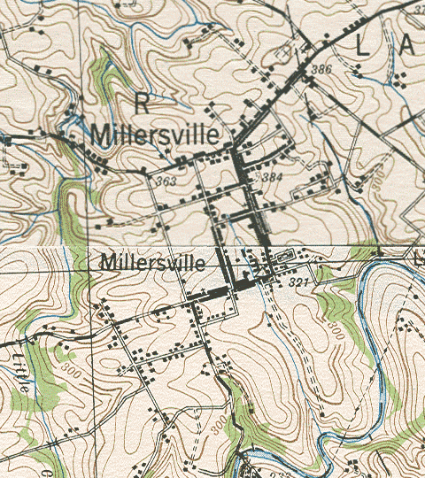
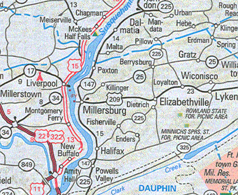
These important concepts were discussed in the context of the longitude-latitude coordinate system back in Unit 2. Here, though, you are asked to recognize the degree to which accuracy and precision depend on the scale of the map. The example used previously was the location of the town of Pillow, PA relative to the border between Dauphin County and Northumberland County. The two maps are shown below. The inaccuracy lies either in a wrong location for the dot representing the town, or the wrong placement of the line representing the county boundary. Of course, we can't know which is right unless we find yet another map, or some other documentation, that shows which side of that boundary Pillow is on.

Interestingly, both maps could still be considered "accurate" by US federal government standards. Starting in 1941, the federal government established accuracy standards that maps would have to meet in order to be labeled as "accurate." In a 1999 USGS version of the standards document, titled "Map Accuracy Standards" (US Bureau of the Budget), Standard 1 says, "For maps on publication scales larger than 1:20,000, not more than 10 percent of the points tested shall be in error by more than 1/30 inch, measured on the publication scale; for maps on publication scales of 1:20,000 or smaller, 1/50 inch." Both of our Pillow maps have a scale smaller than the 1:20,000 scale (a representative fraction scale, which you will learn to recognize shortly), and it is quite likely that the inaccuracy is greater than 1/50 inch (.02 inch). However, if there are only a few errors of that magnitude on the map, the map's publisher is still entitled to print on the map, as stated in Standard 4: "This map complies with National Map Accuracy Standards."

Earlier in this text, you viewed the map legend information information for a USGS digital quadrangle by opening the Attachments list (click on the paper clip icon to the left of the map); in addition to the legend document, there is what is called a metadata document. The main part of the file name of the metadata document is the same as the quadrangle file name but the filename extension is different: XML. It contains the most modern version of that accuracy statement: "This US Topo map product is compiled to meet National Map Accuracy Standards (NMAS). NMAS horizontal accuracy requires that at least 90 percent of well-defined points tested are within 0.02 inch of the true position. In this product, the projection line, grids, and orthoimage are believed to meet NMAS. Positional accuracy of the other data layers is less controllable because of diversity of data sources, and may not meet NMAS. However, other vector layers do generally register well with the orthoimage, which is evidence that the overall accuracy is close to meeting NMAS."

Is this a great failing on the part of our federal government to allow so much error? No, it is simply an admission that they cannot guarantee that every dot, line and patch of color is accurate without spending an excessive amount of money to check.

Determining an Map's Scale

If you have one map with a known scale (or known distances on the ground), and another map or air photo with an unknown scale, you can construct the scale of the latter. You will need to measure the distance between a pair of known features on the map that has a scale and the distance between the same two features on the map or photo whose scale you are trying to determine.

Consider again the basic form of the map scale:

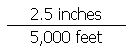
The measurement you make on the map with a known scale plugs right into the ratio we are calling the basic form. For example, let's say that a particular distance between two road intersections on that map is 2.5 inches long and, according to the map's scale, that represents 5,000 feet (how to make such measurements will be shown shortly, if you are unclear about that). We write that as:

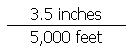
Assume, for example, that the distance between the same two points on the map or photo whose scale you are trying to determine is 3.5 inches. To state the scale of this map or photo, simply replace the numerator with the new measurement. The key concept here is that it represents the same distance "on the ground" for the new map or photo that it did for the first map. So, now the basic form of the map scale of the map or photo whose scale you are trying to determine is:

Map Scale Formats

Verbal and Graphic Map Scales

Remember, however, that the "basic form" is not the format in which the scale will be reported. That format is the topic of the next discussions. In the remainder of this topic you will learn to recognize, measure distances with, and convert between three different ways of presenting map scales. The names of these types of map scales are: the verbal scale, the graphic scale and the representative fraction.

Verbal Scales

A verbal map scale expresses the scale in words. A statement such as "1 inch represents 1 mile" contains both components of the basic form of the map scale. The "1 inch" part of the expression is the map distance, while the "1 mile" part is the ground distance.

You will notice that very few if any of the maps used in this course have verbal scales. They are more commonly used on maps designed for popular publications (newspapers and magazines) or maps in elementary school textbooks.

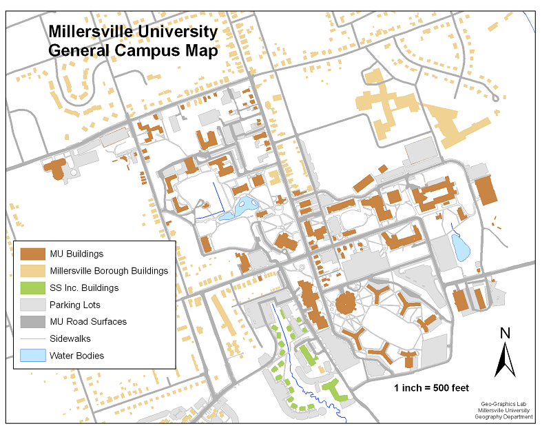
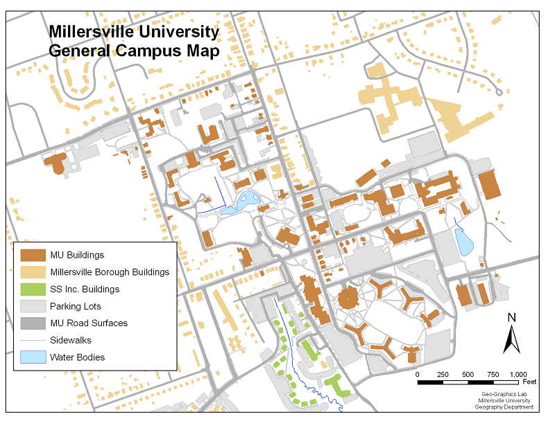
The map below, depicting the MU campus around 2010, is an example showing the use of a verbal scale.

How a Verbal Scale is Formed

There are a few conventions, if not rules, that govern how a verbal scale is presented.

• Both the map distance and the ground distance should be expressed in familiar units of measure.
• The stated map distance should be easily conceived by most map users, as "1 inch" is in our example.
• The stated ground distance depends entirely on the map's actual scale, but ideally it, too, is easily conceived. For example, "1 mile" is better than "5280 feet." If the map's actual scale is "1 inch represents 4879 feet" it is better, if possible, for the cartographer to shrink the map just a little so that a stated scale of "1 inch represents 1 mile" is accurate.
• The word "represents" is preferred over "equals," because it is more accurate (since one inch can never "equal" one mile), although the latter is probably more common.

Making the Measurement

The verbal scale is easily used, as long as the conventions are followed. A ruler is needed to measure any desired distance; that measurement is then multiplied by the stated ground distance.

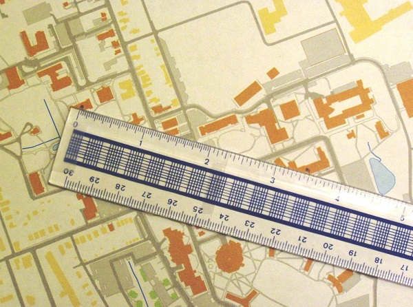
This demonstration will be based on the campus map shown above. The map scale is "1 inch = 500 feet."

The Measurement: Measure the distance between Wickersham Hall and McComsey Hall. This presents one minor conceptual challenge. Since those buildings are large, on what part of each building do you line up your ruler? The answer depends on your purpose in making the measurement. For the purposes of this course, and the safest bet, measure from the center of one object to the center of the other object. You could measure between the nearest corners, or even between nearest doors (if you know their locations), but then you might question whether the building sizes are accurate on the map in front of you. You might then start questioning whether you want a straight-line distance measurement or one that traces a route along sidewalks and internal building corridors. This latter option will be discussed later. To keep things clear, stick with measuring center-to-center.

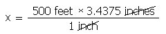
The second map (below) demonstrates that measurement. Note that I am showing you a photo of me making the measurement, rather than offering you a copy of the map to print and measure yourself. That points up another limitation of maps with verbal scales. Computer printers vary, and the various programs used to print graphics can handle the printable area of the page differently, so there is no guarantee that the verbal scale is exactly accurate (it should be approximately correct, though). The measurement is 3 7/16 inches, equivalent to 3.4375 inches.

The Calculations: It is all a matter of proportional relationships. The verbal scale sets up the first part of the equation, to the left of the equal sign. The ruler measurement, since it was made on the map, becomes the numerator to the right of the equal sign. The right side denominator is the unknown in this case, so it will be the answer.

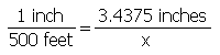
Rewrite the equation with the unknown variable on the left side of the equation and all of the known values on the right. Check the units to make sure that the units of the answer make sense.

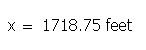
Finally, the answer is (almost one third of a mile):

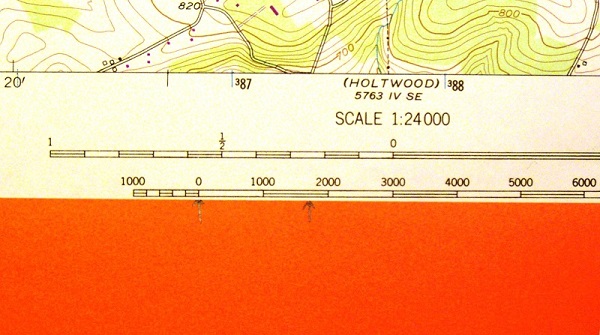
Graphic Scales

The graphic scale form of a map scale is sometimes also referred to as a bar scale or line scale.

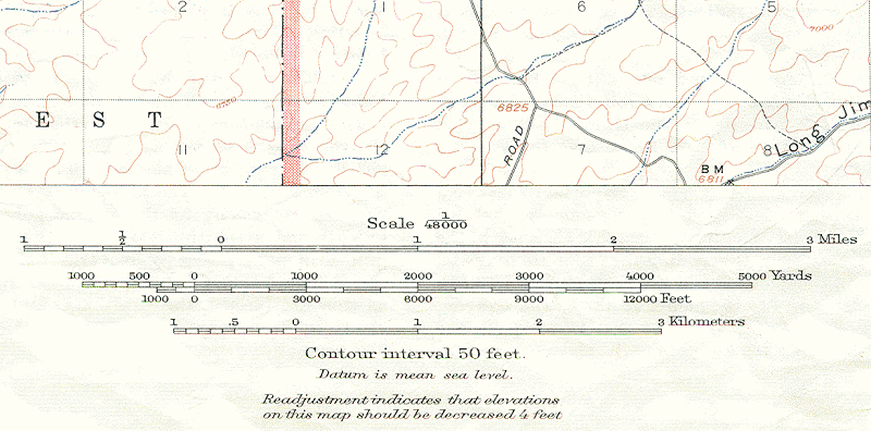
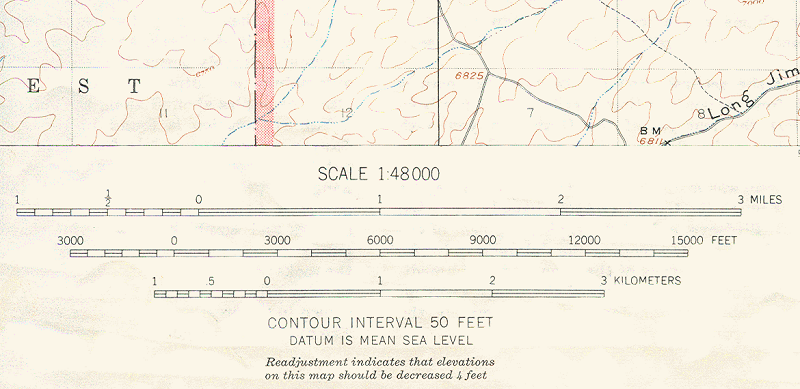
The graphic scale represents the map distance by the actual dimensions of the scale diagram, and represents the ground distance by the labels on the scale diagram. The image below shows the three graphic scales presented on USGS topographic quadrangles.

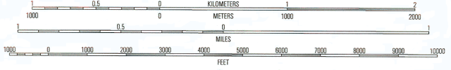
How a Graphic Scale is Formed

The construction of the graphic scale, like all map scales, begins with the information contained in the basic form. The first step is to draw several consecutive horizontal line segments at lengths according to the basic form's map distance. The second step is to label them according to the basic form's ground distance.

Notice in the image above, that the "0" for each different graphic scale is not at the left end of the scale bar. The section of the scale that is drawn to the left of "0" is known as the fractional part of the scale. The fractional part consists of one line segment length, positioned to the left of "0," subdivided in an easy-to-understand way.

Measuring Distances with Graphic Scales

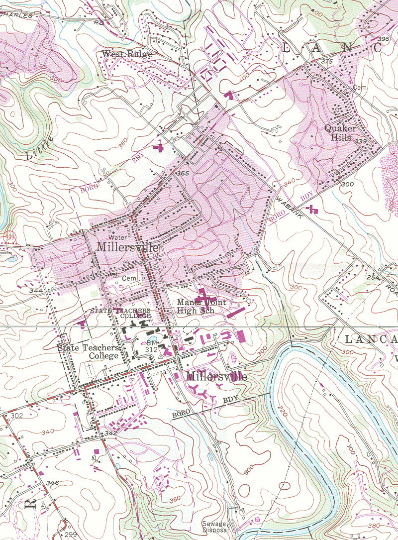
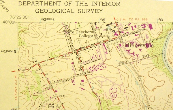
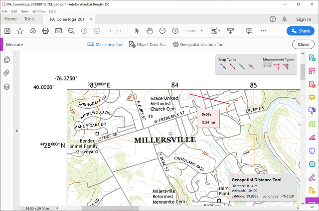
One benefit of the graphic scale is that the map user does not need a ruler. The scale itself is the ruler. The map user does need the edge of a piece of paper. Simply line up the straight edge of a sheet of paper to touch both points and mark those points on the paper. Then line up the edge of the paper with the graphic scale. Here are the steps explained a little more fully, in the context of measuring the distance between MU's Wickersham Hall and McComsey Hall. This time, however, the measurement is being made on a USGS topographic quadrangle. The Millersville University campus is split between two maps, with both Wickersham and McComsey located on the Conestoga quadrangle.

• Find the Points: Locate the two ends of the distance you want to measure. The date of the version of the Conestoga Quadrangle shown is 1990, a photorevision of the 1955 quadrangle. That means that buildings that existed in 1955 are printed in black, but buildings built between 1955 and 1990 are printed in purple. Examine the portion of the campus that appears on this map for a few minutes. Can you find Wickersham and McComsey? What other differences do you notice?
• 
• Mark the Points: Line up the straight edge of a sheet of paper to touch both buildings and mark the center of each building on the paper. Remember: measure center-to-center unless there is a good reason for doing otherwise.
• 
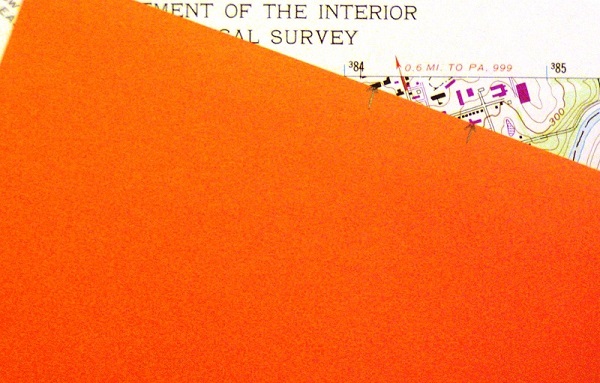
• Line up the Marks: Shift the paper down to the map's graphic scale; in this case, since the map has three of them, we will use the one that shows lengths in feet. Line up your left-hand mark with the scale's "0." It gets a little more complicated when the distance you want to measure is longer than the graphic scale itself, but it is easy enough to add marks to your paper edge (between your marks) that show the parts that the scale does let you measure.
• 
• Realign the marks: You will very likely still have a bit left over, but lining the left-hand starting point of that part of the paper with the scale's "0" gives only a very rough approximation, so we will use the fractional part of the scale. It takes a little practice to get used to using the fractional part; its location left of "0" on the map scale is the key. When a marked length on your paper edge does not end on a scale mark (it rarely does), shift the paper to the left until the right-hand mark lines up with a labeled position on the scale, and read the fractional part of your answer from the "fractional part" of the graphic scale.
• 

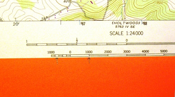
Compare this answer with the one from the previous measurement between the same points. Notice that the graphic scale gives you a less precise answer.

Converting Scales from One Form to Another

Converting a Verbal Scale to a Graphic Scale

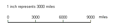
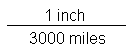
If you have a map with a verbal scale, but would prefer that it had a graphic scale, the latter is easy to construct. The first step is to work backwards from the verbal scale to the map scale basic form. As an example, let's say we have a world map on 8.5" x 11" paper with a verbal scale that says the equivalent scale shown in the basic form is:

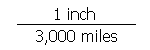
From that information a graphic scale can be constructed. In this case the graphic scale would simply consist of several consecutive 1-inch-long segments labeled 3000 miles, 6000 miles, etc.

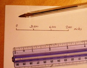
Converting a Graphic Scale to a Verbal Scale

Now let's say that you have the opposite situation, a map whose graphic scale is to be replaced by a verbal scale. Start by measuring the length of the graphic scale's segments; if they are an easy length, then the process is easy. If the segments are an awkward length, then some extra calculations, and decisions, are required. For our (easy) example, let the segments be one inch long and labeled in increments of 3000 miles. So, now the basic form of the map scale starts the same as in the first example:

As long as the lengths and units of measure are appropriate, the verbal scale is simply the basic form's map distance and ground distance are formed into a sentence: "1 inch represents 3000 miles."

Adjusting a Graphic Scale to Show Rounded Values

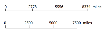
Sometimes, in trying to give a map a graphic scale, the numbers turn out to be a little awkward. It may occur because the map scale is unusual to begin with, such as a scale that was dictated by the paper size, for example: 1 inch represents 2778 miles (which you get if you fit a world map on 9 inch wide paper). That would look rather awkward if used as the graphic scale, as depicted here:

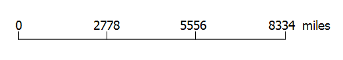
Even though the scale is accurate (correct) it is less usable than one featuring rounded numbers. Remember that graphic scales are not designed to be used with rulers because the graphic scale is the ruler. Therefore, it does not really matter what the map measurement (the numerator in the basic form of the scale) is; the more important value is the ground measurement (the denominator).

The solution:

The solution is to set up a simple equation in which the left side is the basic form of the original map scale. The right side of the equation is another basic form of the map scale which reflects the need for more easily understood labels. In other words, the labels can be rounded numbers such as 2500, 5000, 7500 and 10000 miles. To allow our calculation to work, the denominator of the new (right side of the equation) expression of the map scale will be 2500. The numerator of that right side of the equation is the unknown that the equation will be solved for. So, now the equation is:

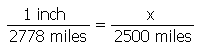
The unit of measure of the unknown is inches because that was the unit for the original map measurement component of the scale (the numerator). Solving for that unknown gives us an answer of 0.9 inches. This means that the lengths of the segments making up the graphic scale will be 0.9 inches each. Whether or not the depiction of that scale (below) is exactly the right size (differences in computer monitors and browsers are almost impossible to account for), hopefully you realize that these segments are a little shorter than the ones above, and that the more rounded label numbers are a lot more acceptable.

Representative Fraction Scale

The Question of Units

The representative fraction scale presents the proportional relationship between map and ground distances in a different way. Even its name is deceptive, although during the first part of the twentieth century this type of scale was actually written on USGS maps as a fraction. The first example below shows that earlier version of a representative fraction scale; the second example shows its more modern expression. In both cases, the way to say the representative fraction scale shown is "one to forty-eight thousand." (Both examples are from older quadrangles depicting the Grand Canyon.)

As with the basic form of a map's scale, the first component of the representative fraction scale is a distance between two points on the map (representing visible locations on the ground), and the second component is the distance between those points "on the ground." The first component is always a "1," and no units are ever stated. Therefore, the literal translation of the representative fraction scale of 1:48,000 is: "one unit of distance on the map represents 48,000 of the same units of distance on the ground."

You Choose the Units

The lack of stated units of measure may be confusing initially, but in fact makes the representative fraction scale more universal than the other ways of expressing map scales. The key is to recognize that the map user must assume that the map distance and the corresponding ground distance are measured in the same units. Thus, 1:48,000 can mean that one inch on the map represents 48,000 inches on the ground, which would be preferable for American map users, but can also mean that one centimeter on the map represents 48,000 centimeters on the ground for audiences in the rest of the world.

Of course, neither 48,000 inches nor 48,000 centimeters is a distance that is easily conceived by anyone. Below, we will review how to make measurements and express the resulting distances in units that make more sense.

Where Have You Seen this Used Before?

The representative fraction is actually a way of reporting scale (notice that I did not say map scale) that is commonly used. Anyone who has played with toys, or made a serious hobby of collecting certain realistic scale models, has probably seen them. Below is a link to a list of examples (Wikipedia contributors).

Determining a straight-line distance using a map's representative fraction scale starts with measuring that distance on the map using a ruler.

The first decision, which is related to that measurement, is whether your goal is a distance in metric units (usually kilometers) or in English units (usually miles). If you decide that your answer should be in kilometers, it will be easier if you make the initial map measurement in centimeters. If you decide that your answer should be in miles, it will be easier if you make the initial map measurement in inches.

Once the measurement is made, the scale must be applied. Remember that the value after the colon in the representative fraction is telling you how many times bigger the real world is than the map. If that map scale is 1:24,000, then multiply the measured distance by 24,000; a measurement of (for example) 2.8 inches on the map is, thus, equivalent to an actual distance of 67,200 inches.

Using a Representative Fraction Scale

Conversion Factors: Of course, 67,200 inches is virtually incomprehensible to most people. That is a common reaction to that first calculation in using a representative fraction scale to determine a distance. The conversion of that value to units that are more comfortable is the next, key, step. To accomplish this next step, you call into use your own knowledge of measurement conversions, as discussed earlier. Assume that we need to stick with English units, so that you will have to convert inches to miles. Remember, there are 63,360 inches in one mile.

There are two approaches to resolving this calculation that are commonly taught. One approach says that you divide 67,200 inches by 63,360 inches per mile. The answer will be the measurement in miles. The second approach says that you multiply 67,200 inches by 1 mile per 63,360 inches. The answer is the same; the only difference between the two is that one or the other will mesh with how you have been taught and what you feel comfortable with. The key to success using either approach is keeping track of your units of measure as you proceed through the calculations.

Standard Representative Fraction Scales

USGS Map Standards: The USGS was named the lead agency in the US government's National Mapping Program in 1975. One purpose of the program was to standardize map production through many different government agencies, from the US Census Bureau and the US Department of Defense to the US Geological Survey itself. Many map products were already in circulation, so decisions were made about which products to continue and which to abandon. Larger scale maps were in increasing demand.

Remember, from our discussion of the basic mapping process, that the decision of which map scale to employ actually reflects two decisions: how much of the Earth's surface (in this case) to depict, and what size paper (again, in this case) to present it on.

Standard USGS Surface Areas

The USGS decided that the different map series would cover:

• One degree of latitude by two degrees of longitude.
• One degree of latitude by one degree of longitude.
• Thirty minutes of latitude by one degree of longitude.
• Thirty minutes of latitude by thirty minutes of longitude.
• Fifteen minutes of latitude by fifteen minutes of longitude.
• Seven and a half minutes of latitude by seven and a half minutes of longitude.

There were many exceptions made, for a wide variety of reasons, but this list at least demonstrates the objective.

Standard USGS Distance Scales

The USGS decided that the map sheet sizes would reflect these standard representative fraction scales:

• 1:250,000
• 1:125,000
• 1:62,500 (although there were some maps at 1:63,360 and some at 1:48,000)
• 1:24,000 (although there were some maps at 1:25,000 and some at 1:31,680)

The main products were 7.5 minute quadrangles at 1:24,000 scale; 15 minute quadrangles at 1:62,500 scale, 30 minute quadrangles at 1:125,000 scale, and 1 degree quadrangles at 1:250,000 scale. All of these combinations produced sets of (approximately) rectangular maps which covered the entire US, and some of other areas. Smaller scale maps at 1:500,000 scale and 1:1,000,000 scale could have continued the series established by the first three scales listed above. 1:62,500 was also chosen because it was approximately 1:63,360 (one inch represents one mile). 1:24,000 represents a departure from that sequence, but was preferred because at that scale one inch represents 2,000 feet, a nice round number. For a while in the 1960s and 1970s it was planned that 1:24,000 scale maps would be replaced by 1:25,000 scale maps, which were better suited to metric distance calculations at a time when there were attempts afoot to change the U.S. to a metric country, but obviously that has not materialized. (Thompson 1981, 20-26)

A Few Other Interesting RF Scales:

Globes: Globes are among the smallest scale maps. Remember that globes are the only maps for which the scale is true on every part of the map.

• One globe with a diameter of 12 inches has a scale of 1:41,849,600 (it also has a verbal scale of '1 inch represents 660 miles').
• A second globe with a diameter of 12 inches has a scale of 1:41,817,600 (while its verbal scale is also '1 inch represents 660 miles').
• A globe with a 16-inch diameter has a scale of 500 miles per inch, which corresponds to a representative fraction scale of 1:31,680,000.
• A globe with a 24-inch diameter has a representative fraction scale of 1:21,100,000.

Remember that the diameter of each globe must be multiplied by pi (3.14159) to calculate its circumference; that circumference then corresponds to the length of the equator, which on the Earth is about 25,000 miles.

Classroom Wall Maps: These maps are on large sheets and cover varying amounts of the Earth's surface, so there is a large amount of variation. The widths reported here are just the width of the land area shown, not the total width of the paper.

• One wall map of Japan and Korea, which is 76 inches wide, has a representative fraction scale of 1:1,000,000.
• A 43.5 inches wide wall map of Australia and New Zealand has a representative fraction scale of 1:6,000,000.
• A wall map of Asia, from the Middle East to the Phillipines, 48 inches wide, has a representative fraction scale of 1:9,200,000.
• A wall map showing the entire Eastern Hemisphere in an area 76 inches wide has a representative fraction scale of 1:10,000,000.
• The continental United States depicted on a 62-inches wide wall map, has a representative fraction scale of 1:3,000,000.
• Showing the entire world on a wall map that is 59.5 inches wide results in a representative fraction scale of 1:23,800,000.

This list of wall maps shows a great variety of areas covered and their corresponding representative fraction scales, to give you a 'feel' for the kinds of numbers involved.

The more you see maps and take note of their representative fraction scales, keeping in mind the areas they depict and their sizes as presented, the better you will understand what the magnitudes of those scale values represents in terms of detail and larger versus smaller scales.

Converting Scales from One Form to Another

Converting a Verbal Scale or Graphic Scale to a Representative Fraction Scale: If you have a map with a verbal scale or graphic scale, but would prefer that it had a representative fraction scale, the latter is easy to construct. The first step is to work backwards from the verbal scale or graphic scale to the map scale basic form, which you have already learned to do. As an example (the same one used in demonstrating the conversion of a verbal scale to a graphic scale, and back), let's say we have a world map on 8.5" x 11" paper with a verbal scale that says "1 inch represents 3000 miles" or the equivalent graphic scale consisting of several consecutive 1-inch-long segments labeled 3000 miles, 6000 miles, etc.:

From that information determine the map scale's basic form.

The procedure, then, requires first that you ensure that the numerator of the basic form fraction is a "1" with known units. The second step is to convert whatever value occupies the denominator of the basic form fraction to the same units of measure as the numerator. Since the example already shows 1 inch in the numerator, it is merely necessary to convert the denominator, 3000 miles, into inches. Depending on your preferred procedure, the conversion requires that you either divide 3000 miles by 1 mile per 63,360 inches, or multiply 3000 miles by 63,360 inches per mile. The result is the same either way: the numerator remains one inch while the denominator is replaced by 190,080,000 inches. The final step is to re-write the basic form as the representative fraction 1:190,080,000. Compared to the USGS standard scales, the number after the colon in that answer is huge. Remember that in basic (fraction) form, the larger the denominator is the smaller the total value of the fraction is; in terms discussed earlier, the larger that value after the colon is the smaller scale the map is.

Converting a Representative Fraction Scale to a Verbal Scale or Graphic Scale: Now let's say that you have the opposite situation, a map whose representative fraction scale of 1:190,080,000 is to be replaced by a graphic scale or verbal scale. In this case, stating the basic form of the map scale starts is a challenge because it is necessary to assign distance units to the numbers, the same units applied to the numerator and denominator of the basic form. Since we already know the equivalent scale in inches and miles, let's create a verbal scale and a graphic scale in metric units. Thus, our conversion from the basic form starts as:

As we have seen, the key now is to convert the denominator value into metric units that are easier to visualize than 190,080,000 centimeters. Longer metric distances are usually expressed in kilometers. Since there are 100 centimeters in a meter, and 1000 meters in a kilometer, the conversion is 100,000 centimeters for each kilometer. Since 190,080,000 centimeters is in the denominator of the basic form expression of the map scale, and we want the kilometer measurement to be in the denominator of the next illustration of the basic form scale, multiplying by 100,000 centimeters per 1 kilometer yields the following:

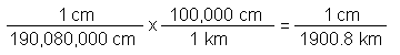
The statement "1 centimeter represents 1900.8 kilometers" would then be placed on the map. Of course that is a little awkward because 1900.8 kilometers is not easily visualized. If you were committed to a world map on conventional printer paper, you could shrink the map a small amount (which could be calculated) so that a "1 centimeter represents 2000 kilometer" verbal scale is accurate.

Converting the same initial basic form expression of the map scale to a graphic scale requires the same initial calculations as determining the verbal scale. However, in the resulting scale, one centimeter segments are rather short and 1900.8 km, 3901.6 km, etc. are rather awkward labels. As we learned during the discussion about graphic scales, it is rather easy to set up an equation to figure out the equivalent scale that has more comfortable values and units. In this case, let's decide to create a graphic scale that has segments labeled in 5000 km increments. How long would the segments have to be? That means that the numerator should be the unknown in the equation. Setting up and solving the equation yields the following:

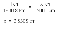
The solution there is the basic form scale needed to construct the graphic scale. Draw segments that are 2.6305 cm long and label them with multiples of 5000 km.

Scale and Zooming in Map Software

On-line map sites such as Google Maps allow you to zoom in or out on the map. One way is to use the computer mouse's scroll wheel. The online maps generally also have a pair of icons on the map itself labeled with a "+" and a "-" that can also be clicked on to zoom the map. Google Maps does have a very short graphic scale on its interactive maps; it is not much good for measuring distances on the map, but it can give a sense of the magnitude of those distances. These characteristics are pretty much universal among all the online interactive map sites.

Zooming in this fashion makes the map larger or smaller. The features on the map get closer together or farther apart. Zooming is something that most people do with these online interactive maps without thinking. We must recognize that the zooming process is actually the process of changing the scale of the map.

The Adobe Reader Measure Tool

Adobe Reader added its map capabilities only in the last couple of decades. Before that, the functionality of the "GEO-PDF" was available using an add-on program that worked within Adobe Reader called the TerraGo Toolbar. If you download older scanned versions of the USGS quadrangles, dated before 2000 for example, you may be prompted to download the toolbar; do not do it, since the Adobe Reader "Measure" tools take care of those tasks now. Adobe's technique for changing the scale of the map is based on its ability to change the relative size of the document page. Adobe indicates the page's relative size as a percentage. To zoom in you must change the percentage to a higher number, and to zoom out make the percentage lower.

Since you are using Adobe Reader to view professionally created maps, you have one way to convince yourself of the scale changes. Move the map view to show the graphic scales below the map area of the USGS quadrangle. Change the percentage page size and watch the length of the scale bars (as measured with a physical ruler) change.

Zooming by percentage in Adobe Reader means that you never really know the scale of the map as you are looking at it. Even when the zoom level is set to 100%, it is difficult to be confident that the printed scale on the map matches the scale of the map as displayed on your computer screen. From that information and our earlier discussion about scale types, the only valid map scale to use in that environment is the graphic scale.

Scale and Zooming in ArcGIS

As you learned when you were first introduced to ArcGIS, GIS programs also allow users to zoom in and out of a scene. As a standard feature in all GIS programs, it is typically performed using menu icons such as "Zoom In," "Zoom Out" and "Full Extent" tools and using the scroll wheel on the standard computer mouse.

Since we now know zooming to be a process of changing the scale of the map, how does ArcGIS let the user keep track of that scale? ArcGIS Pro displays the current scale of the map as a representative fraction in the lower left corner of the main map area of the window. Watch it change as you manipulate any of the tools just mentioned. The user can also type the portion of the map scale that comes after the colon, or click on the downward-pointing triangle to the right of the map scale and choose a new scale from a list. Note that these map scales appear in the software but not on the map itself. ArcGIS does have a way to add a graphic scale to the map, which will be described later in this text.

The same caveat applies to ArcGIS's displayed scale that was mentioned for Adobe Reader's percentage "scales." In relative terms scale adjustments will be accurate, but the only way to know whether the displayed scale is absolutely accurate is to make map and ground measurements and do the calculations to confirm (or not) that scale. Your computer's graphics capabilities and your monitor's pixel resolution can affect the results.

Measuring Distance and Area

Measuring Distances

You have seen how to measure straight-line distances using the three types of map scale: verbal scale, graphic scale and representative fraction scale. There are several concepts to keep in mind while doing so.

First, remember that every paper or other "flat" map is a distortion of the true surface of the Earth, and only on map projections of the Equidistant category will your distance measurements be consistently accurate. Every other category of projection will distort distances, especially if they are longer distances or distances that are relatively far from the areas of tangency of that projection. The Equidistant projection maps are all in the polar planar category, and the distances that will be consistently accurate have to pass through the central "polar" point of the map, so even those maps are not to scale in all areas of the map.

Second, when you are measuring the distance between two map features, consider what "between" represents. When travel companies tell you the distance between two cities, they have usually identified a central point in each city to measure those distances to and from. If you are asked to measure the distance between two buildings for this class, I will specify a similar center-to-center measurement.

Measuring Great Circle Distances

Back when we were being introduced to the concept of Map Projections, we looked at nine characteristics of the Earth or a globe. One of those characteristics involved the concept of a Great Circle. It was described as any circle, such as the equator or any meridian and its opposite, which, if we cut the globe on that line, would give us two equal halves of the globe. You also saw the observations that any two points on the Earth's surface determine one unique great circle and that the path of the great circle between those two points is the shortest distance between them. The only exception to these rules is if the two points are on absolute opposite points on the Earth. One example (out of an infinite number of possible examples) of this scenario is the North Pole and South Pole; we already know that there are an infinite number of possible meridians between those two points.

Let's call those two points A and B. Another way to describe the Great Circle defined by any two points on the globe is that it is the circle constructed as a perfectly flat plane through the Earth that includes three points: the two surface points A and B between which we are measuring, and also the center of the Earth. The intersection of this plane and the Earth itself is the great circle defined by points A and B.

Once you have that concept of a great circle, then you can show the distance, D, between the two points as an arc, like this:

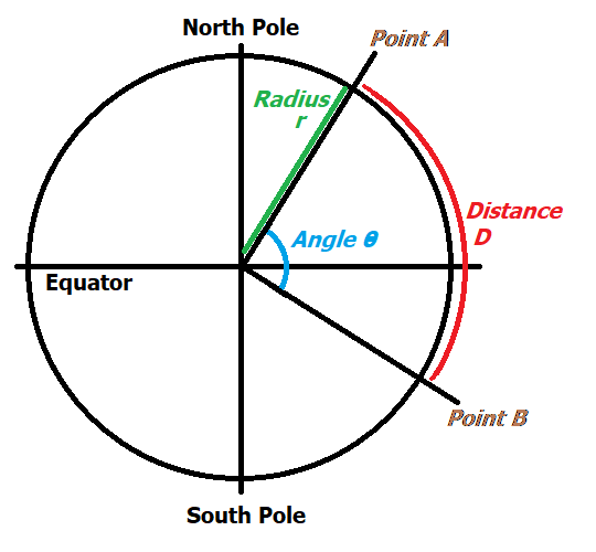
The outer black circle represents the Earth, whose circumference, c, is equal to the expression 2πr. The "r" value is the radius of the Earth. The Earth is not a perfect sphere, but pretending that it is introduces less than 0.5% error. Well-established approximate values are 25,000 miles for c and 8,000 miles for r.

We can also observe that the complete angular circumference of a circle is 360°. Between points A and B on the surface of the Earth we can construct the angle they form with the center of the Earth, which we can call Θ (Greek letters like "theta" are usually used to represent angles). If we measure our angle Θ using a protractor, we can compare that angle with 360°. Calculate Θ as a percentage of 360° then our desired distance D is that same percentage of the Earth's circumference.

The angle Θ would be easy to calculate if our two points on the Earth's surface were directly north and south of each other, in other words if they fell on the same meridian, which is what the diagram above is really showing. In that case the angle Θ is easily constructed using the latitudes of points A and B. However, since that is not likely to happen, calculating Θ becomes much more complex, requiring the use of trigonometric functons. There are such formulas for calculating Θ that use the latitudes and longitudes of points A and B, though the level of math required to use them is beyond the scope of this course.

Measuring the Length of a Line that is Not Straight

Most of the time we are using maps to measure distances, the path from one end of the distance to the other is not straight. The best examples are measuring the distance to be covered in a road journey, or measuring the length of a river or a boundary.

Unfortunately, you will probably never make an accurate measurement of those distances with a map. The only way to get it right is to travel the path on the Earth using some sort of measuring device. Using maps, including computer-based maps, will almost always underestimate the distance.

One "low-tech" method for measuring such distances is to lay a string following the path on the map, marking the endpoints of the path on the string, and then picking the string up and using the map's scale to measure and convert that length. The limitation of this technology, the only one likely to overestimate the distance, is that all forms of string or rope are likely to stretch a bit when straightenend for measurement. The fibers that give the string its flexibility to bend as needed also give it a tendency to stretch.

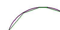
The other technologies for making this measurement tend to rely on breaking the path into short straght segments, and then adding the lengths of each segment to form a total. As the drawing below illustrates, the straight segment will always be shorter than the actual path, unless that path is perfectly straight.

Computer-generated maps and distance measurements fall into this trap, too, because of the way the paths of roads and rivers are stored digitally. Any line is stored in memory as a series of points, to be connected by straight line segments when the line is drawn. The point locations are stored using their X and Y coordinates, the nature of which depends on the projection/coordinate system combination established by the users of the computer's cartographic software. The coordinates might be in decimal degrees, in UTM meters, or in State Plane feet, for example. The lengths of degree-based segments would have to be calculated using standard conversions. The distance from every point to the next is then an application of the Pythagorean Theorem.

Some computer maps will be more accurate than others. They achieve the improved accuracy by using more points to represent the line, essentially breaking the path into shorter and shorter segments. The costs of achieving this improved accuracy include a greater amount of memory required to store all of the points, a greater number of calculations to make the length measurement, and consequently a longer processing time (you may not notice the time if you use a powerful computer) to find the answer.

There is one device which measured curving paths on maps without breaking them down into short straight segments: the "map measurer" or "measuring wheel." You may have seen a full scale version of this device used to measure lengths at a construction site or to mark the yard lines on a football field. The map version is smaller but still relies on a geared wheel dragged along on the map tracing the desired route while the wheel's circumference measurements are shown on a dial. The devices were great, in theory, but relied heavily on the quality of the map and on the user's steady hand.

Measuring Distances in Map Software

Measuring Distances using Adobe Reader

Adobe Reader includes a "tool" for measuring distances on USGS quadrangles. The icon to initiate the tool, called the Measuring Tool, is found in the same group as the Geospatial Location Tool used previously to find precise latitudes and longitudes on a quadrangle. The capabilities of the Measuring Tool are tied to the fact that the quadrangle open in Adobe Reader has a set map scale (1:24,000 for the maps we have used the most) and has set page dimensions.

When you click once on a starting location, and then click once again on a destination point, a red line will be drawn and the information box in the lower right corner of the window within the program will display the distance, along with a smaller popup box near the distance line. Changing the units of measure for the measured distance is as easy as right-clicking anywhere within the map area of the window. The choices are displayed once you click "Distance Unit" at the top of the menu that opens.

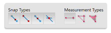
There is another aspect of the use of the Measuring Tool that users ought to be aware of because it influences the accuracy of the measurement. When the tool is open a second smaller window appears in the upper right area of the map window. It has two groups of icons, one group labeled Snap Types and the other labeled Measurement Types. The default Measurement Type will measure Distance (the other two types will be discussed below). Snap Types refer to the fact that the map is drawn in Adobe Reader the same way ArcGIS draws maps, one layer at a time. Each layer of features consists of points (for point features) or points that are strung together to make lines (for line and area features), and "snapping" means that any place you click near an existing feature on the map for your measurement will be moved to the nearest existing point. If you are not trying to click on an existing point but happen to click near one, the cursor will be moved away from the point where you actually clicked. Most of the time, that behavior will be annoying, and you will want to turn it off. Use the Snap Types icons to do so simply by clicking on those icons. Here are those icons in their "on" position, which will cause snapping to occur.

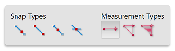
And here are the icons after all were clicked "off." Generally, it makes the most sense to either keep them all on or all off, although of course there could be exceptions.

Another distance measurement scenario is measuring the total length of a path that has several turns in it. This requires clicking on a beginning point, clicking on each consecutive turning point, and then double-clicking on the ending point. The first tool, as just described, cannot handle that scenario. The second tool in the group of tools in the upper right corner of the map is the "perimeter tool." This tool can be used to capture the length of the perimeter of an area, but it also works for this purpose of capturing the length of a non-straight line.

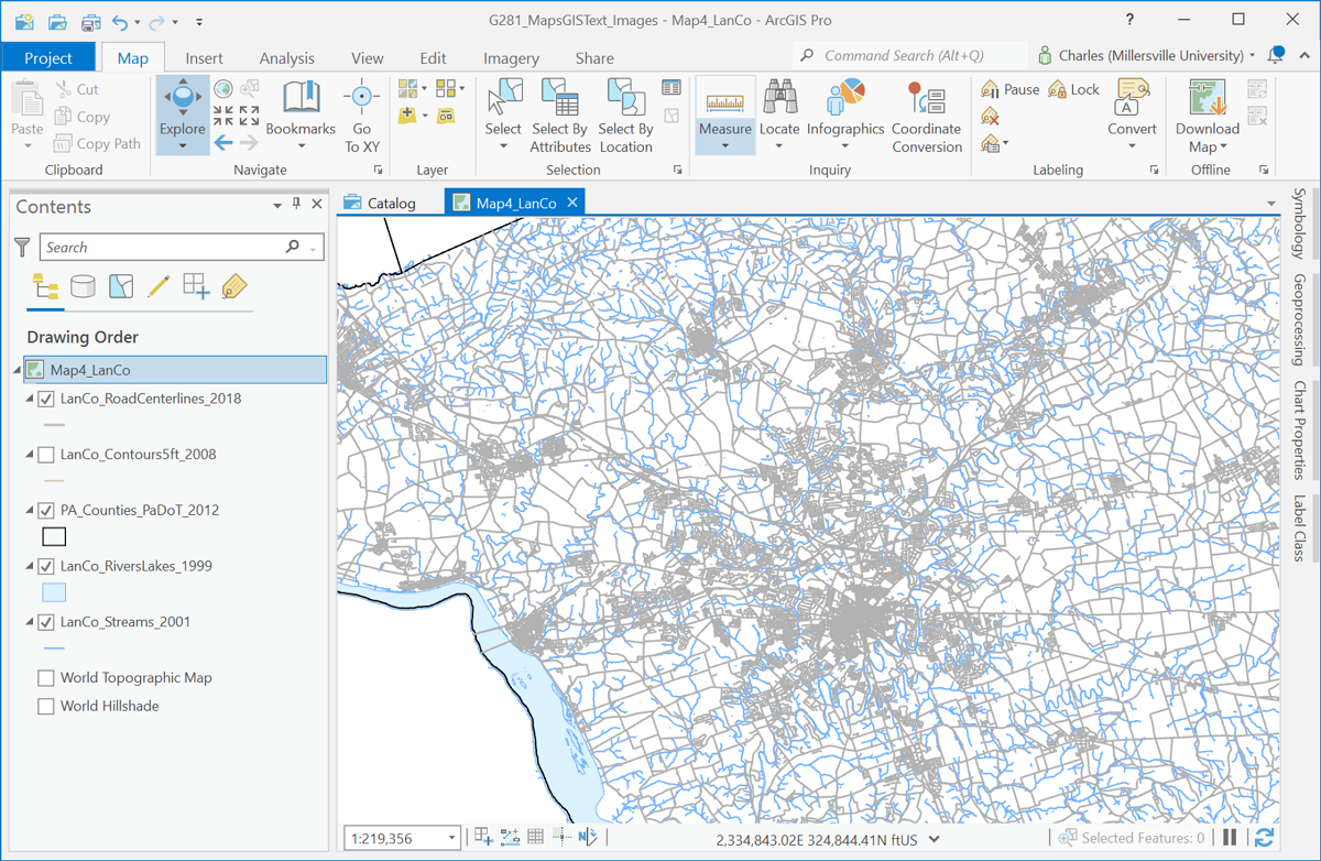
Measuring Distances using ArcGIS

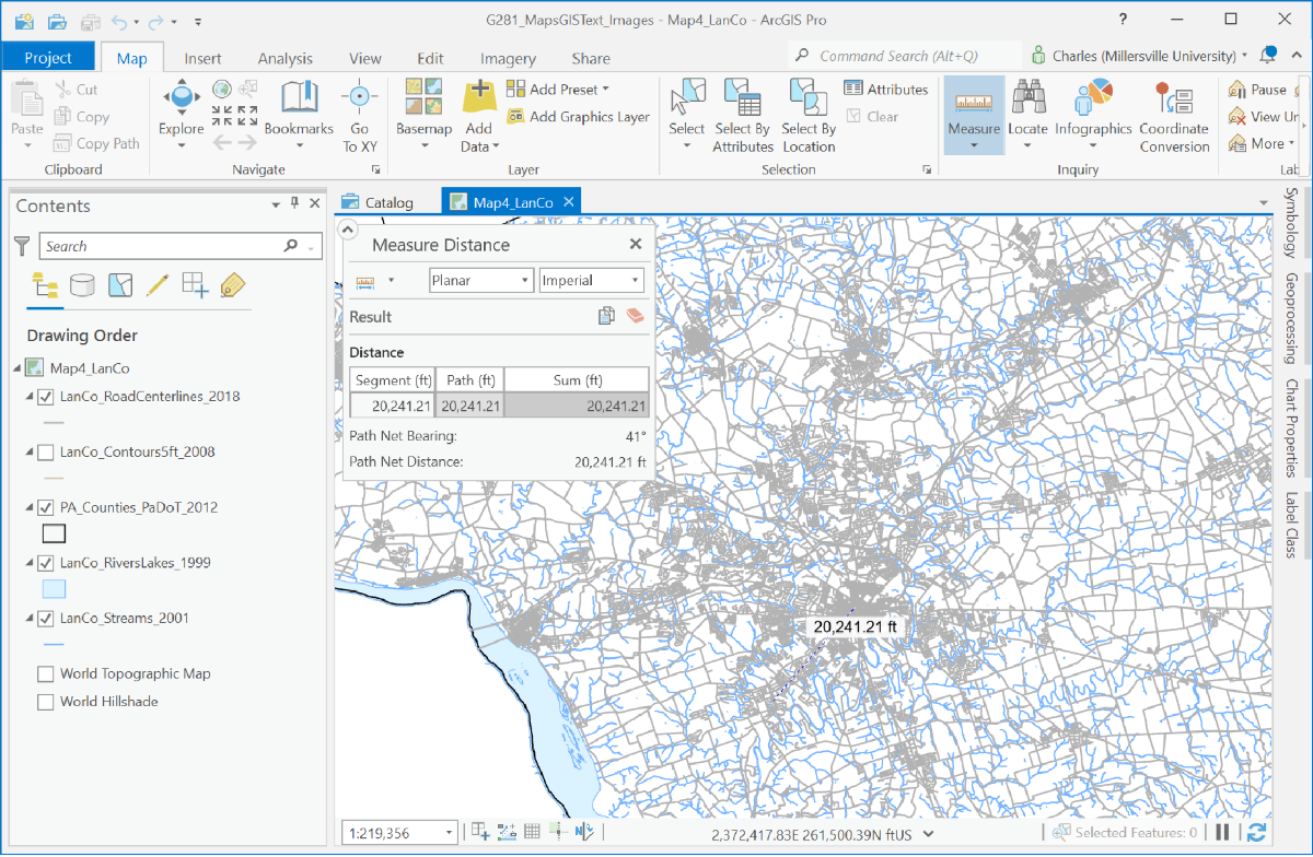
In ArcMap the task of measuring a distance is performed with the "Measure" tool, which allows you to click on two or more points and then tells you the total distance through all those points. In other words, the default behavior of the ArcGIS measure tool is the same as Adobe Reader's distance tool and perimeter tool combined. The "Measure" tool icon is: . The Measure tool is on a menu ribbon above the map, as shown below. Like the perimeter tool in Adobe Reader, when you click once on a starting location, and then double-click on a destination point, a line will be drawn and an information box will pop up to display the distance. In ArcMap, that information pop-up has a spot to click on that will open to a list of other units of measure, so they can be changed "on the fly."

In GIS software, the programmers assume you are trying to be precise, so their formulas account for the precise locations clicked. Distortion due to the roundness of the Earth or due to the current map projection must be accommodated, but when zoomed in on a smaller map area the distortion is less significant. The distance measurement shown above for such a larger scale is called a "Planar" measurement. When zoomed out, however, the curvature of the round earth and the map projection are more significant factors. The Planar measurement type can be replaced by one that incorporates those factors. "Geodesic" is the best choice in those situations.

Measuring Areas

Visualizing Areas to Measure

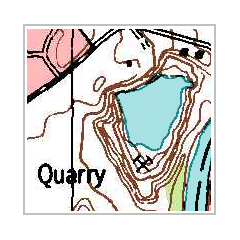
Map features whose areas you might need to measure include lakes, watersheds, surveyed properties, city blocks and even large buildings. Remember that areas are always reported in "square units;" for example, one square mile is any shape that covers the same area as a square that is one mile long and one mile wide. Here is an example we will follow:

Measuring Simple Shapes

In school you have seen how to measure the area of simple shapes in plane geometry. You may even have memorized the formulas for the area of a square, a rectangle and a triangle. Be prepared to brush up on those formulas as needed.

One approach to measuring the area of a more complex shape is to break it down into smaller pieces that are simple shapes. A combination of squares, rectangles and triangles, however small, may give a good approximation of surface area covered by some features. After using your basic geometry formulas to measure the area of each smaller piece, add them together to get the total area.

Measuring Complex Shapes

There is no foolproof way, or mathematical formula, to measure the area of a highly irregular shape, and most natural features such as lakes and swamps, will be of that type. The best one can hope for is a good approximation. There is a mechanical device, called a polar planimeter, that uses some geometrical principals to give a very good approximation. However, like the linear "map measurer," its accuracy depends on the user's steady hand and consistency, which are difficult to accomplish.

The most common approach to measuring the area of a more complex shape is the same one mentioned above: to break it down into smaller pieces that are simple shapes. The most common approach is to break them down into one type of shape, the square. Your television and computer monitor do this when they break an image down into pixels. This approach works best when all of the squares are the same size, and are small relative to the total feature size. In fact, the smaller the squares, the more precise the total measurement will be.

You can imitate the digital process if you have to measure a feature, for example our lake, on a paper copy of a topographic map. Simply lay a piece of graph paper over the feature (the lake). Next trace the lake onto the graph paper. Count the squares that are completely inside the lake. Then count any squares along the edge of the lake that have more than half of the square covered by the lake; ignore the squares that are less than half covered. The principal is that the non-lake areas in the 'more than half covered' squares will be nearly equal to the lake areas in the 'less than half covered' squares. Again, for greater precision and accuracy, the smaller the squares the better. Use your map scale to measure the area of one graph paper square, and multiply that area by the total number of squares counted.

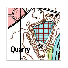
In this example there are 67 full squares and 17 squares that are more than half covered by the quarry lake. Each square is 80 feet x 80 feet in area. Therefore our estimated area of the lake is 84 x 6400 square feet = 537,600 square feet.

Area Measurements in Map Software

Compared to the measurement of linear distances in online interactive maps and map software such as Adobe Reader and ArcGIS, the measurement of area is less common. Area measurememnt on USGS quadrangles in Adobe Reader is done in a clear but somewhat limited way, and in ArcGIS there are several types of area measurements offered.

In Adobe Reader, as noted above, the Measure tool has an option for measuring the Perimeter of an area; it also has an Area tool (in the same group of tools) for measuring an area that you outline with successive mouse clicks. As each is selected, the contents of the information box in the lower right corner of the Adobe window changes. The difference with measuring the perimeter of an area feature is that you must make the final double-click on the same point you started on. The same procedure applies for using the Area measurement tool. Additionally, the same advice about turning off all the snapping options applies for area-based measurements.

There is one limitation to the Adobe tools. If you want to know the perimeter and area of the same outlined area, you will have to click that outline separately for each measurement. Of course, it will not be easy to click on exactly the same points.

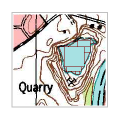
In the case of the lake described above, the image below shows the area measured with the Area measurement tool. The dialog shows the area measured as 0.2 square miles. Converting that to square feet gives a total of 557,568 square feet.

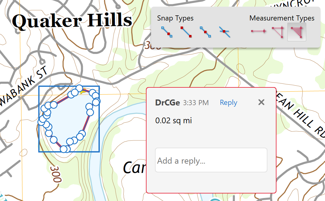
In ArcGIS Pro, the same tool used to measure distances also measures areas, perimeters and other types of measurements. We will take a closer look here, because there are some features which make it a little more complex.

The ArcMap Measure tool has multiple options as shown below. They are made possible by the fact that the software maintains so many detailed measurements related to layers and features. If you choose "Measure Area,"" it works like Adobe Reader in that you click on the points to create your own temporary area, but the information window shows both the area and perimeter measurements. Once you double-click to finish the measurement, the measurement information remains in the information window. As with the Distance measurement tool, the information window gives you the ability to change the units of measure and to make allowances for the curvature of the Earth.

A more useful option of the Measure tool for the purpose of our example here is the option to "Measure Feature." All you have to do is click cleanly on the desired map feature, such as our lake, and the information window will be filled in. Here are the results of measuring our lake feature: the total of 528,453 square feet is close to our previous estimates.

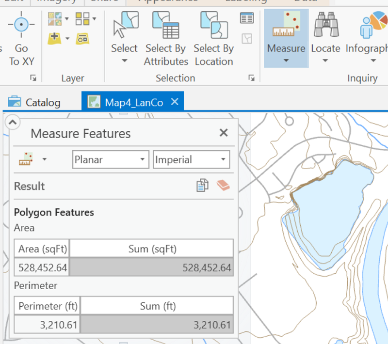
Even though the three measurements reported above for the quarry lake were not exactly the same, the differences were modest. There are many sources of difference between them, such as the ability to control the mouse clicks, the detail with which the software captured the measurements and even rounding error within the calculations. A range of less than 30,000 square feet out of over 500,000 square feet amounts to only about 5% error.