Transportation

Roads and Highways

Our first transportation topic is roads, with railroads entering this discussion below. Later in the unit, in our discussion of economic activity, we will mention some characteristics of ship activity.

Road Symbols and Jurisdictions

The USGS Roads Legend: The legend that differentiates different road symbols and the different route number categories is the only symbol legend that appears directly on USGS topographic quadrangles.

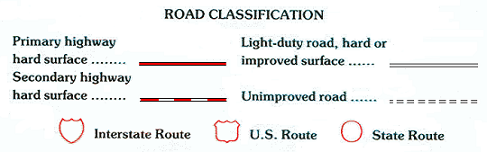
The four types of roads symbolized and named in the legend were subjectively defined. It is probably easy to think of examples from your home town that fit the four levels of road types, but defining the precise difference between primary and secondary or between secondary and light-duty is not simple. It can also depend on the type of area the map covers: smaller back roads in a densely built-up area might not be shown, but a road made the same way in an isolated rural area might be important locally so it would be shown.

When examining roads on USGS quadrangles, keep in mind that the scale width of a standard two-lane road (one lane in each direction) is wider than its actual width as measured on the ground because the USGS has adopted a road symbol that is sized to be easily visible, not to be accurately scaled. Four-lane and wider roads can therefore be shown with accurately scaled widths.

The route number symbols are very specific. Interstate Routes are a different system from the US Routes, and are represented by their actual highway marker symbols, but both were built and are maintained by the federal government. Each has an independent route numbering system, which will be explained presently. State Routes are also given route numbers but, were built by their respective state governments. Each may have their own route symbol shape, like Pennsylvania's keystone shape, but the USGS chose to represent them generically with the circle symbol.

The rest of our road system consists of roads under the jurisdiction of lower levels of government, from the states to the counties to the local municipalities. Usually, the decreasing level of government reflects a decreasing level of traffic, but there are many significant exceptions, especially near major cities. A relatively small number of the more significant roads are labeled with their names.

An example of a type of local road with high traffic is the number of small to medium cities and towns that have pushed major roads onto by-passes around the city or town. By-passes were seen as necessities to keep through-traffic from congesting the center of town. Other development issues accompanied that trend, as we shall see below.

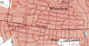
The Jurisdiction Hierarchy: The road network today consists of several levels of road quality (as shown in the legend above) and of road connectivity. These relate to who paid for the roads to be built and who maintains them. At the most local level are private roads, not shown on most maps. These are roads that are contained within large, essentially privately-owned properties and were built and are maintained by their owners. University campuses and farms are two examples. In the map of Lancaster County, Pennsylvania below, none of these are represented (not that you could have seen them if they were).

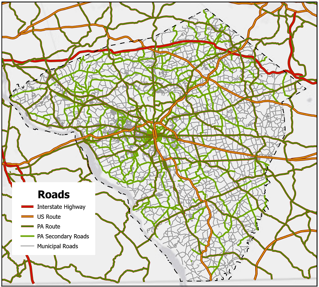
At the next level, in suburban housing developments, towns and cities, and even in very rural parts of the countryside, are the back roads and side streets. The municipal level of government (township, borough or city) is usually responsible for these smaller roads. The urban and suburban streets were often built by developers and then turned over to the municipality. In the map above they are shown in gray.

At the next higher level are county-owned roads and secondary state-owned roads; they are shown on the map by solid green lines. These still tend to be smaller roads but are primary routes connecting smaller towns within the county.

The final parts of the color scheme on the Lancaster County map are the three types of highways. They will have been built by the federal or state government as primary and heavy duty travel routes. They will be the subjects of the discussions below.

Roads and Highways

Roads serve at least two transportation-related functions. First, they provide for local circulation, to give city dwellers access to their homes and businesses. This means that with dense development there has to be sufficient access for the volume of traffic needed to distribute all goods and services. The second function of roads is to connect distant places. The most efficient connection is usually the shortest, but landscape challenges such as water bodies and rugged terrain must be taken into account also. These functions demonstrate that you cannot talk about roads and transportation without taking into account the people and places they serve and the natural landscape they cross.

Historical context is important, especially regarding roads. Many of our current connecting roads follow the same alignment as original dirt roads created hundreds of years ago. Many such roads that have to be re-built to meet modern demands and standards are problems because there is no room to make the road wider, since they are roads designed for long ago when populations were smaller and vehicles were slower.

Historical Development of Highways: Major roads can be readily dated using several factors:

• Many towns/cities and roads date back to colonial times, and some are even older.
• Most US towns/cities were planned before they were built.
• Early roads connected town centers and formed center-of-town blocks.
• Industry increased population growth and transportation needs, which were served by railroads and roads.
• It took several decades after cars arrived for them to become widely used.
• The first national highway building project built the US Highways.
• Second national highway building project built the Interstate Highways.

The first few factors in the list above refer to early roads. Keep in mind that they were little more than dirt trails serving travelers on foot, on horseback, and on wagons, even in the largest cities of that period. Those same pathways today are buried beneath layers of concrete and macadam, today's roads. In other words, for most of our history, what came before worked just fine for the next big thing in transportation.

That reluctance to change was altered significantly with the introduction of railroads in the second half of the 1800s, but mostly for the railroads themselves. New routes were found, or made. The shortest path was not necessarily the best because trains traveled so fast (even then), but it had to be as gentle a slope as possible because of the weight they pulled.

The US Highway System

Automobiles arrived toward the end of the 1800s, but their competition at that stage was the horse and the pedestrian, not the railroads. In other words, they were primarily used for local circulation, not for long distance travel. Road paving was not seen as important until after World War I, and even then it was simply the paving of the old dirt roads. The early US Routes were built in the 1920s and 1930s, partly to put men to work during the Great Depression. Their function was still to connect city center to city center. They had at-grade intersections with every road they crossed. US Route 30 is a local part of that system, and up until the late 1950s Route 30 followed King Street and Columbia Avenue right through downtown Lancaster, and followed Market Street through York. Of course there were fewer cars and trucks on the roads in those days and their top speeds were much slower than today.

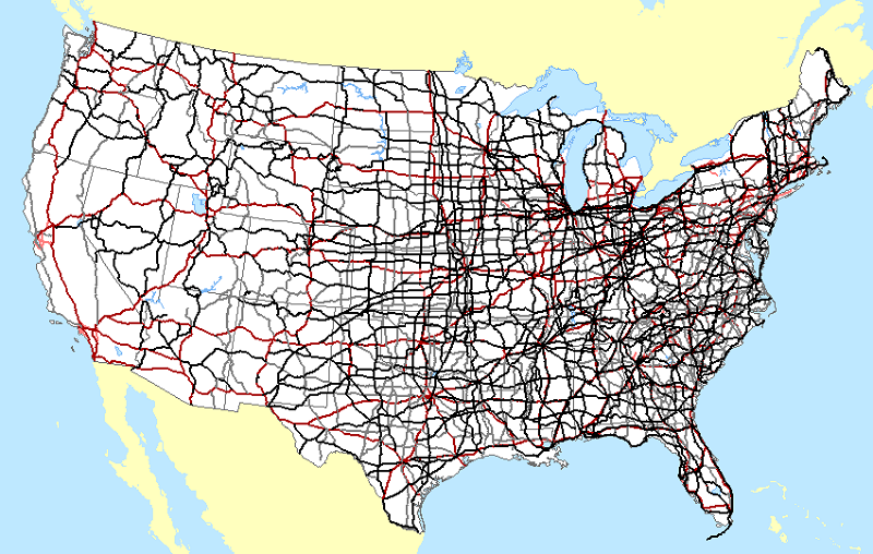
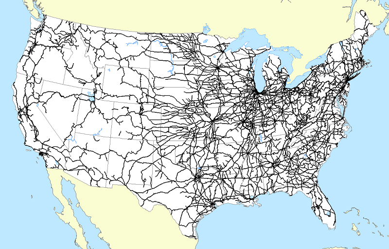
The level of service they provided meant that there had to be many US Highways. Connecting so many medium and large cities, and trying to avoid missing any of them, was a significant challenge. And then, once the major routes were constructed, the secondary US Highways were built for greater interconnectedness. The map below shows the highways of that network.

An innovative feature of the US Highways system was its route numbering scheme. The map shows the north-south alignment of some routes and the east-west alignment of most others. The major routes were given two-digit route numbers. The north-south routes were given odd numbers with the lowest numbers in the east (US Route 1 goes through Boston, New York City, Philadelphia, Washington, DC and Miami) and the highest in the west. The east-west routes were given even numbers with the lowest numbers in the north (for example, US Route 6 across northern Pennsylvania) and the highest in the south. These highways are symbolized with black lines on the linked map. Once the two-digit US Highways were designed and largely built, the federal government funded secondary roads connecting with those US Highways. These were assigned three-digit route numbers with the same-shaped sign. This map shows these in a gray color.

Interstate Highways

The modern era in highway building coincided with the decline of the railroads, with a defining moment occurring here in Pennsylvania. In the 1880s the New York Central Railroad tried to retaliate against a territorial intrusion by the Pennsylvania Railroad by starting construction on a new line across southern Pennsylvania. An economic recession and intervention by the government convinced both companies to abandon their projects. The Pennsylvania state government acquired the New York Central's track bed but did not use it until the late 1930s. Looking for a way to improve highway travel, they built the first section of the Pennsylvania Turnpike on the old railroad bed. It was the first long-distance limited-access highway in America. It set the design standard later adopted in the construction of the Interstate Highway system, and later became Interstate 76 (or I-76) in that system.

The design standards for the Interstates include limited access ramps, wide lanes, gentle slopes (mostly 2 percent or less), and barriers between opposite-direction vehicle lanes. Every road that crosses the path of an Interstate Highway is put on an overpass or in an underpass. The route numbering system was similar to that of the US Highway system, with even two-digit numbers on east-west routes and odd two-digit numbers on north-south routes. The order changed, though, with the lowest route numbers in the west and south, and the highest route numbers in the east and north.

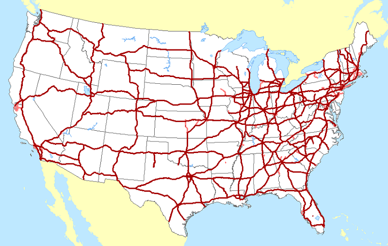
Both the US Highways and the Interstate Highways are still maintained. In fact many miles of US Highways (and of other state and local roads) have been upgraded to Interstate Highway design standards. In the Interstate system, as in the US Highways system, additional connecting highways have been built with three-digit route numbers. In the map below, the two-digit-numbered Interstates are represented in dark red, while those labeled with three-digit numbers are shown in a lighter red.

Railroads Today

Mainly because railroads were still the largest carrier when the US Geological Survey was gearing up its mapping of the country, most railroad facilities are mapped in great detail. In addition to the inter-city freight and passenger transportation of its early years, railroads spawned the development of intra-city transit systems. The features of those systems are represented inconsistently on USGS maps, though.

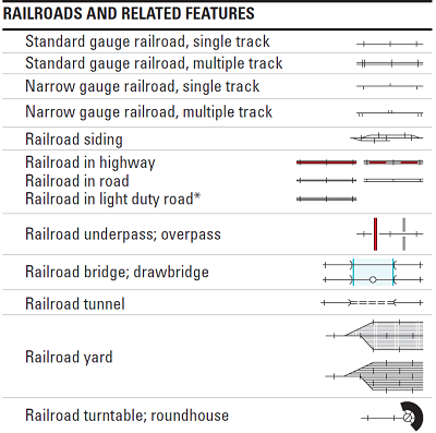
The main component of the railroads is the tracks, of course, and the legend shows the attention that was paid to the number of parallel tracks as well as the "gauge" of those tracks: "narrow gauge" refers to a closer spacing between the rails, sometimes used on smaller branches of the network. Note that the representation of railroad tracks suffers from the same scale problem we saw with road symbols: the width of the standard track symbol is not a perfectly scaled representation of the actual track's width. Also key are the "yards" of many tracks crowded together; they help with storage of extra railroad cars, and the sorting of cars into trains. Passenger stations, warehouses, train construction and repair facilities, and "roundhouses" for storing and maintaining train engines are common building structures along railroads.

The location of railroad facilities in and around cities is generally associated with their industrial activity, which we will see more of later. Passenger stations are located within business districts, since their primary customer base are now the commuters between city and suburb.

Even though railroads do less business than they used to, they are still a critical part of the transportation system. Whenever raw materials are produced from farms, mines, and forests, given the bulk and quantity of those goods the railroad is the cheapest way to transport them any significant distance. The same can be said for high volume outputs from factories. The only cheaper system is water-borne transportation, but there are fewer opportunities for that.

The difference between railroad transportation and other forms is best measured in tons per mile. The quantity of diesel fuel (the fuel of diesel train engines), the small crew to run a large train, and the durability of tracks and the "rolling stock" (engines and cars), are much cheaper than hauling the same quantity on many trucks, each with its own fuel and driver costs. Airplanes are even more expensive than trucks. Again, ships on the oceans and barges on larger rivers can be cheaper, but they travel more slowly than railroads.

One example of the efficiency of railroads was the Pacific Fruit Express system, which peaked in the 1930s to 1950s. A cooperative venture of two western US railroads, it ran refrigerated trains from the west coast to anywhere in the country. When California became a major agricultural producer, the Pacific Fruit Express could deliver picked produce from the west coast in refrigerated cars to the big cities of the east coast within two days.

Development

Development History in the US

What is Development?

The development process always begins the same way, even today. Someone (an individual or group) does the following:

• buys (or proposes to buy) a large piece of land,
• draws up a plan to divide the property into smaller properties,
• gets permission to proceed,
• has the roads and other infrastructure built,
• may build on each property, or may offer them "unimproved,"
• and starts selling.

The properties are developed either for housing, commercial or industrial purposes. The properties destined to become schools, churches, parks and other public or quasi-public uses are more likely being "developed" by governments and non-profit organizations than by developers (or the developer is required by the government to add those uses to his plan).

In colonial times in the eastern part of the US, the developer most likely bought from the colonial government, whereas in the rest of the US the developer most likely bought from the federal, state or territorial government. On the other hand, today, the large piece of land is more likely to be bought from a farmer or similar rural land owner. Following the same process, smaller properties can be bought for individual (residential or commercial/industrial) development.

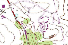
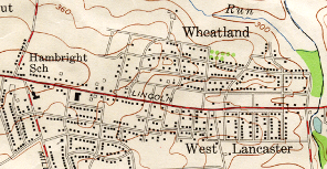
On USGS quadrangles new developments are visible in a few different ways. For one, if the same quadrangle is obtained for several different dates at least a general idea of the age of a development as long as it occurred within that time span. A second clue applies to the older paper versions of the quadrangles in which purple symbols of all kinds (roads, buildings and other features) are used to represent features added based on aerial photography evidence obtained since the map was last "ground checked." It was a quick way to identify somewhat newer developments, but not really reliable if the map had been photo-revised for several consecutive editions; it also disappeared as an clue if the map had been field-checked. Finally, occasionally a newer development would show up as roads with an apparently incomplete collection of buildings, as in the example below.

Historical Context

The first task is to put the key stages and events into historical context. Think of this in parallel with the transportation history we examined above.

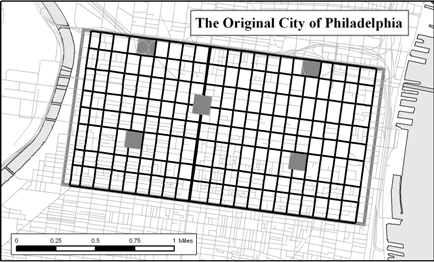
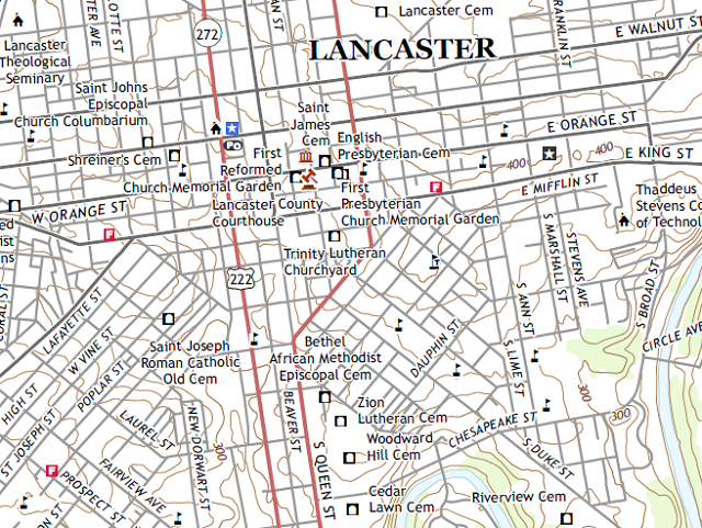
Early Development William Penn was the first colonial governor to create his principal city according to a very strict plan. Even though his plan of "what should go where" was not adhered to, the grid pattern of streets became the norm in city planning. Older cities like Boston (the original downtown section) are not structured in that way; their main streets are more likely to follow the original wagon paths that preceded the city. Following Penn even small towns are likely to follow a grid plan, unless they grew without a plan. Unplanned towns grow by the individual purchase of many small properties with no strong leadership or coordination.

The map below, of Philadelphia, shows the part of the city that William Penn laid out as the rectangular grid of streets. On the "Boston South" USGS quadrangle (see the download recommendation below), look in the northeastern area--but not in the corner--of the map. The area around City Hall was the extent of Boston in colonial times. That immediate map area shows the disorganized street pattern of an unplanned city.

USGS Quad to download and examine:

Boston South, MA
(7.5 x 7.5 minutes)
Look at the street patterns of the oldest area of the city of Boston, compared to parts of the city that were built later.

Development Stages: Even though the process for creating developments has not really changed in hundreds of years, the goals of development (beyond that of making money for the developer) have changed. Development can be readily dated in this regard using several factors:

• Remember that the first settlers encountered a completely undeveloped landscape in colonial times.
• Early livelihoods were primarily based in subsistence agriculture, so towns were smaller, fewer in number and pretty well spread out.
• Cities and larger towns grew most rapidly during industrialization, in the late 1800s and first few decades of the 1900s.
• The rapid shift to suburban population growth did not occur until after World War II.
• Urban areas (that is, a city together with its suburbs) continue to grow even though the city itself is most likely losing population.

City Structure

Background

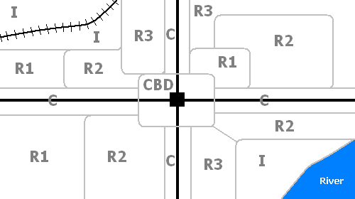
Urban places that are fortunate in their location, whether due to transportation access, nearby resources, local investment, or many other possible factors, will grow. Also, following the success of William Penn's Philadelphia street plan, older cities and other unplanned towns that continued to grow almost always grew by adding gridded extensions. That practice continued up until the late 1940s. Cities tend to have cohesive business/government, residential, and industrial districts. The locations of some of these districts may evolve over history, but their cohesiveness is likely to persist. Follow the diagram below as we examine these land uses.

we will take each of these districts in turn and identify map clues that help us to find them. Look at this with two cautions in mind. First, definite boundaries of these districts will not be easily determined; rather, the best you can do most of the time is to identify the heart of each district. Second, with the advent of suburban growth, as we shall see presently, many of the functions that these districts served have been attracted to locations outside of the city itself. The result has been that cities are now faced with either redesigning the district to serve another purpose or trying to attract a new generation of landowners to the existing structures there. Those processes are not readily seen on the traditional topographic maps, but the aerial photographs on the newer digital quadrangles can show them very clearly.

The CBD

To start, almost any small town (and even the large cities, as originally planned) has a major road or intersection of roads that defines the "center" of that town. Around that center, the land will have the most potential value: prime real estate. That downtown district is the best location for the most money-intensive organizations, and it is also the best location for government operations that oversee the town and its surrounding area. It is referred to as the Central Business District (CBD; see the diagram below), but is actually a business-and-government district. It frequently will also feature some other old and venerated institutions in the town, such as the library, the theater or opera house, and the older, wealthier churches.

Other areas of the city are primarily commercial, without having the high land value or the tall buildings of the CBD. These commercial areas (labeled C in the diagram) generally line the main roads into or out of town.

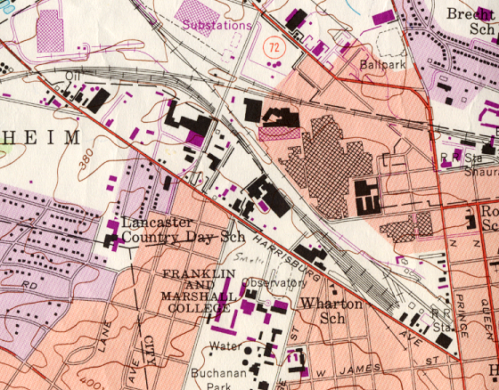
The CBD is visible on topographic maps using several clues. Within the reddish or pinkish "urban tint" or "house omission area" only landmark and government buildings are shown. So, look for City Hall, the Courthouse, the Library, a concentration of churches (usually the oldest and most traditional denominations) and similar structures. The Post Office ("PO" on the map) is normally marked there, too, because it was originally a purely governmental function; however, in many cities the main postal processing center has moved out to the suburbs. The roads may also be a significant clue, since the main roads of the center of town are likely to be given higher traffic designations and have highway-type route numbers labeled.

Industry

Part of the town or city will likely be industrial; since the late 1800s that was the economic foundation for most places. Industry needs heavier-duty transportation than the original crossroads could provide, so the industrial district will be centered a port, a railroad yard or, nowadays, an Interstate highway exit. Water has the added attraction for industry of being a coolant for energy-intensive operations. Some cities are large enough to have multiple industrial districts.

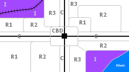
The industrial district will be visible primarily because of the transportation access. Look for railroad tracks and storage yards (many parallel tracks), railroad sidings or spurs, docks and dredged water channels in a bay or river, and Interstate highway ramps. Older paper maps showed industrial buildings outside of the urban tint areas, but on the later paper maps the urban tint areas were often extended to include industrial districts. Not all industrial buildings, as big as they usually are, were considered to be landmark buildings. Lancaster's industrial districts have been transitioning to other uses in recent decades, so the best way to see local examples would be to examine older Lancaster, PA USGS quadrangles for evidence of the industrial districts in the northwestern and northeastern quadrants of the city.

Aerial photographs can be more useful than topographic maps for detecting industrial areas. The buildings will be visible, of course, especially given their large size. More importantly, though, the means of transportation, and some of the inputs, equipment and finished products will be easily seen outside the buildings. Neither the older nor newer USGS topographic maps symbolize parking areas, for example, but a large fleet of trucks parked in a large lot stands out very clearly on aerial photos. Lancaster city's railroad tracks have been removed from the industrial areas they used to dominate, so they are not part of the more recent quadrangles. Even so, the presence of railroad tracks on a topographic map does not guarantee that they are still in use, especially given the industrial decline occurring in major cities of the northeast. The air photo layer can show whether those railroad sidings are being used if they are still well stocked with rail cars. Again, in Lancaster's case the older scanned paper quadrangles, or older aerial photographs show a strong railroad presence. In Lancaster's case the railroads were essential because it is an inland city with no major river connection.

Residential Areas

Urban residential areas generally have no obvious clues for identification. Sometimes well-known neighborhood names will be printed on the map. Most, especially in larger cities, will feature their own neighborhood schools (shown on USGS quadrangles), as well as grocery stores and other services (not shown on the USGS maps) for neighborhood residents. Other than that, you are usually looking for street characteristics (width and spacing) and areas that are not the CBD or industrial districts.

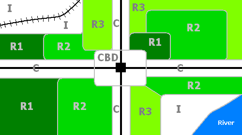
Near the CBD will be a residential district (R1 in the diagram above) that caters to the wealthier people who work in the CBD. Even though many of them may now live on more open properties in the suburbs, the dwellings they originally built in the city will tend to be large and stately. The roads through these districts will also be broader, and they are likely to feature alleys where their horse stables (in the 1800s) or multiple-car garages are hidden from public view.

Industry employs many lower-income workers, and the residential areas for them (R3 in the diagram above) are usually near the industrial districts. The housing that they can afford is smaller, which is reflected in a higher density of dwellings (most likely row-homes) and more closely spaced and narrower streets. More difficult to see on USGS topographic maps, but easily seen via the advertising markers that pop up on Google Maps, is that these residential districts are likely to form neighborhoods whose populations have consistent ethnicities and income levels.

Note that I have not talked about a middle-class residential district. The middle class is really a much more historically recent phenomenon; it did not grow to significant size until after the Great Depression or possibly even World War II in the mid-1900s. That means that it, like the automobile, wasn't really planned into the structure of older cities (Los Angeles is a great exception, though). The era of middle class/automobile-based suburban development will be treated below. In recent years, however, the middle class has been "discovering" city life, and some sections of the city--usually the best of the lower class districts (R2 in the diagram above)--have been renovated for their use.

Finally, you should be aware of the re-development efforts of the 1960s to 1990s. Much of the redevelopment was aimed at updating commercial areas of the city, but a significant effort was put into improving living conditions for the poor. Some was misguided, however, and resulted in unappealing "housing projects" (many were high-rise apartment buildings) that have aged much more poorly than the housing they replaced in some respects.

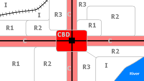
The Suburbs

What are Suburbs?

Suburbs have generally been added in newer and newer rings around the town or city, concentrating first at the major road arteries leading into the town or city. Some suburbs date back to the end of the 1800s when the wealthy moved to estates outside the (then) city boundary and commuted in by streetcar. Cities and towns of that era generally grew by developments which added a few more blocks of gridded streets to one edge area of the place. Usually, the city boundary was extended to include that development, so we often do not recognize it as a suburb today.

The growth of what we now recognize as the suburbs really started after World War II. Factories, residential developments and then commercial developments abandoned the city for newly developed land just outside. The causes were many: decay in the inner city, the building of by-passes to relieve city traffic congestion, and increasing city taxes to pay for increasingly expensive services.

In the diagram below, the by-pass is the focus of commercial (C) and industrial (I) development. Residential areas (R) fill in the areas between major roads, offering their residents space, but creating a planner's nightmare: suburban sprawl.

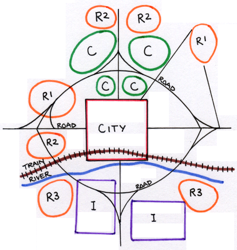
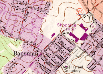
Levittown, NY, followed by Levittown, PA, set the mold for the modern automobile suburb. They were initially designed for lower middle class families whose head would be working at a nearby suburban industrial site, and who had probably been in World War II (receiving government post-war benefits), and who had probably previously lived in the city. They were designed with car ownership in mind and with no urban-style row homes or semi-detached dwellings. The homes were also designed for mass production, and developed in great numbers around every city and every significant or successful town. Their automobile orientation led to suburban shopping centers or plazas and other sites with large parking lots (again, the parking lots are not visible on topographic maps, but are clearly visible on aerial photographs).

Suburban Street Patterns

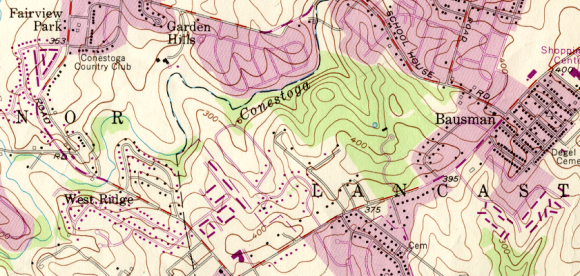
The street patterns of the earliest suburban developments were somewhat gridded, but had somewhat curving streets. This design persisted through the 1950s and 1960s. The example below is from the 1997 Lancaster, PA USGS quadrangle.

By the 1970s developers had learned some lessons about car speed hazards to children in the developments, and began introducing design changes to make the neighborhoods safer. In the 1970s that meant fewer access roads to discourage drivers who were using the suburban grid as a shortcut between main roads. More curviness to the roads also reduced the speed of the cars. The northern half of the map excerpt below illustrates a development of this era.

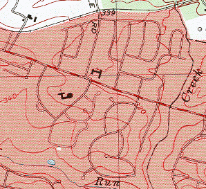
In the 1980s neighborhoods were more likely to feature only one or two access roads and very confusing street layouts. Only people who lived in the development were welcome and would be familiar the easy ways in and out. Also growing in popularity at that time was the inclusion of cul-de-sacs in the street layout. The southern half of the map excerpt just above is an example of a development of this period.

On older topographic quadrangles the streets and each house of a suburban development are likely to be shown. The USGS did not consider them dense enough to include in the urban tint area. Later in the 1990s, their design standards changed and they began erasing the buildings in favor of the urban tint. For that time from the 1950s to the 1990s, though, it is possible to estimate the populations of such suburban developments by counting the number of houses and multiplying the county by an average family size (2.8 is a good average for modern American families). The maps below show one development (the same as the first one above) as depicted on the 1956 and 1997 versions of the Lancaster PA USGS quadrangle.

Other Suburban Developments

Two other housing phenomena peculiar to the 1960s and later are the apartment complex and the mobile home park. An apartment complex is a collection of larger longer buildings, usually rather tightly packed, but on the suburban fringe of the town or city. Again, they are more likely to be visible on older maps, and more likely to be included in the urban tint area today. The example below is from the Lancaster, PA USGS quadrangle. Can you find the three apartment complexes?

Suburban industrial and office parks are another post World War II phenomenon. As noted above, they are attracted toward Interstate highway exits and by-pass exits for truck transportation access, and away from higher city taxes. In some cases, the cities continue to extend their boundaries to include such developments and maintain their tax base, but in other cases the cities lose when such companies flee to the suburbs.

Economic Activity

The Variety of Economic Activities

Economists and economic geographers tend to study economic activities structurally, as indicated in the chart below. Our interest, of course, will be in looking for evidence of these activities on topographic maps.

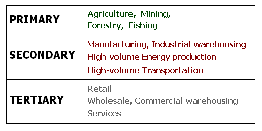
Activities at the primary level have the greatest impact on extensive areas of the surface.

Secondary-level economic activities include manufacturing, energy production, and also transportation, which has already been covered well.

The tertiary level emphasizes retail-wholesale activities and other services.

Primary Level Economic Activities

Agriculture

Farming includes crop growing, obviously, but also includes ranching and other livestock operations. Most of it requires large land holdings, and many involve very specialized buildings to house equipment, store products temporarily, or even to do some preliminary processing of the products. Road access to individual farms is usually not a major concern, but access to railroads in the vicinity is usually important for getting the produce to larger market and processing centers.

We talked about map evidence indicating the presence of agriculture earlier, in considering the representation of the farm fields as a form of vegetation. The farm fields and pastures are represented by white space with a cluster of farm buildings. In naturally forested areas straight edges to the forest represent land areas cleared for crops or pastures. In the central and western parts of the US you can expect the farms to fill US Public Land Survey System quarter sections or other rectangular boundaries.

Orchards, vineyards and cranberry farms (bogs) are examples of specialized types of agriculture that are identified on topographic maps. Ranches and other livestock operations are less obvious unless there are other clues visible on the maps, such as place names and road names.

When using on-line map services, aerial photography may show the farm landscape more more clearly than map views do. Often, though, the aerial photography is taken during the late fall or early spring (the "leaf-off season"), so the best evidence may not be available. Ancillary businesses that are often easily identified on topographic maps and air photos include railroad freight facilities and stockyards.

Mining

Mining also requires extensive areas of land, but in this case the land surface will be greatly "disturbed" as shown in the excerpt from the Mount Carmel, PA quadrangle below. In areas of surface mining (also known as open pit mining or strip mining) like Mount Carmel, deep pits, access roads and even railroads, and areas for disposing of waste materials from the mines are important landscape changes. Underground mines also require waste disposal areas, and will also have several buildings that house elevator and ventilation equipment. The pollution of nearby streams is a significant concern today. Railroad access is of prime importance to get the raw ore to refining operations or manufacturers.

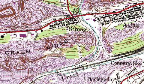
There are many areas of the US in which mining has been a primary source of income for a large part of the population. Such areas make great subjects for study because they tell economic, cultural and environmental stories about those places.

Mount Carmel, PA
(7.5 x 7.5 minutes)
On older versions of the quadrangle, look for the symbols used to portray mining activity, including the purple map photorevisions. On older and newer versions of the quadrangle, look at the town characteristics.

Mines Symbology: Mines had their own set of symbols most of which, once you knew what they represent, were pretty self-explanatory. It remains to be seen whether the USGS will update these for the newer digital quadrangles.

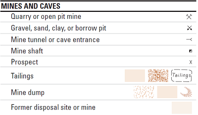
The difference between quarries, mines and pits as surface mining operations is primarily the type of material being extracted, but also can indicate the scale of the operation (quarries and pits being smaller than mines). Underground mines are accessed either by horizontal tunnels (the same symbol used for natural caves) or by vertical shafts. The distinction in the legend between "tailings," "mine dumps" and "former disposal sites" is not important (considering they can all be represented by the same symbol anyway). They are all places where mine wastes are left.

Forestry

Forested areas are clearly present on the USGS topographic maps, obviously, but it is important to realize that not all forests are being harvested for lumber. Evidence that a forest is being cut might include areas of an extensive forest that are now bare, and straight edges of the green forest symbol can represent the cut edge of the forest. Keep in mind that the mapping of forests is based on aerial photographs, and represents just a moment in time, just like the photograph would.

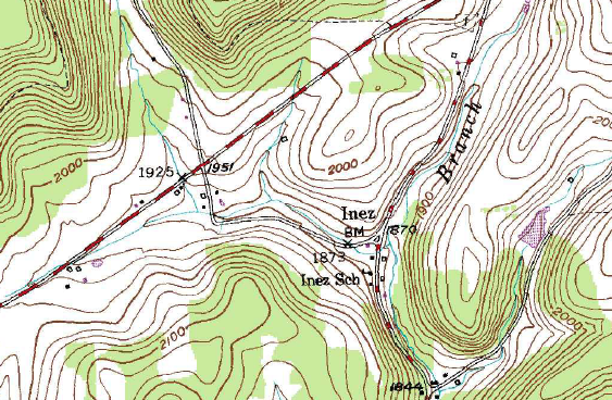
The logging taking place in the area shown above, the village of Inez in northwestern Pennsylvania, is not easily seen on the map, but if you compare it with a photographic view from Google Maps and similar sites you will see that the forests are actually very sparse and heavily cut. Inez is found on the Austin, PA quadrangle.

Forestry operations also depend on those heavy duty trucks reaching nearby manufacturing, railroad or port facilities. Sawmills or pulping mills may be located near the forests, or may be located in a regional industrial center receiving the logs. The railroads and ships could be taking the logs, or the milled wood products, great distances in some cases.

Fishing

Fishing will have relatively little impact on land areas, except that very easily identifiable dock facilities will be needed for the boats. Fishing facilities bring together three related discussions from this unit. First, the boats are significant contributors to the local transportation system, not just for hauling the fish in from the fisheries, but also for sending the cleaned and processed fish, and possibly other local goods, to their destinations very cheaply. Second, the wharves and warehouses and processing plants are likely to make up a significant part of the industrial zone of the city or town. The third discussion to which fishing activity is relevant is coming next: the sense in which the local economy becomes specialized and this activity feeds from the primary level to the secondary and tertiary levels as well.

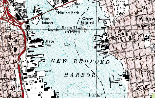
Remember that if fishing is to be a significant part of the local economy, it is by using larger boats and coastal locations by the ocean or Great Lakes. Smaller lakes and other inland waters, no matter how numerous, will at best support some recreational fishing, which does not earn significant income. In those cases the economic geographers will classify the local economy as a "service" type of economic activity.

Secondary- and Tertiary-Level Activities

Secondary-Level Activities: Energy

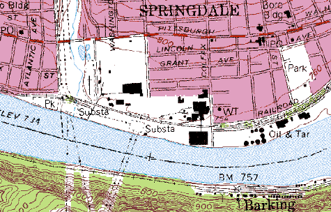
The most significant energy production facilities, other than mines, are electric power plants, many of which are huge in size. Some, however, are small and compact, no bigger than other industries. The power plants that are not hydroelectric, wind-powered or solar need fuel, which means a heavy duty transportation system such as railroads or pipelines (some older USGS quadrangles represented and labeled pipelines, though not consistently). Since the product of power stations is electricity, there will be an electrical transformer substation nearby, with high-capacity transmission lines leaving the area, possibly in several different directions. Again, on older quadrangles both the substations and the high-voltage electrical lines were frequently shown with appropriate symbols and labeled.

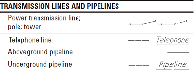
Electric power plants will occasionally be labeled (on older maps, especially) and may show areas of coal piles or oil/gas pipelines. They will generally be large buildings, and will certainly be located adjacent to an electrical substation with many lines representing power lines emanating from the area.

Construction of Dams

Some dams are among the tallest structures humans have built. Like the bridges and tunnels that will be described in the next section of this Unit, their impact by themselves is significant but not overwhelming. Their most significant impact occurs when construction is complete, when the dam is closed and the reservoir fills. The amount of water being stored in the reservoir depends on the height of the dam, the width and shape of the river valley, and the slope of the river being dammed. That reservoir could be short and shallow, but it could also be hundreds of feet deep and extend upstream from the dam for more than a hundred miles.

The recommended example, below, shows the Grand Coulee Dam on the Columbia River in the state of Washington. One interesting exercise to practice with maps that include dams is to determine how the water flows. Which way is the Columbia River flowing through the Grand Coulee Dam? Look at the water level in Franklin D. Roosevelt Lake, the reservoir formed by the dam, and at the elevations along the river "below" the dam (not the mile marker numbers in the river below the dam). Is the town of Coulee Dam safe if the dam breaks?

Grand Coulee, WA
(7.5 x 7.5 minutes)
Look for the dam itself, the reservoir upstream and the river downstream, plus all of the associated landscape elements.

It should also be noted that many smaller dams are not made of concrete, but are constructed and landscaped to blend into the environment. Even though their core is probably many tons of construction boulders and other rock, they are generally covered with earth (and planted with grass), and referred to as earthen dams.

Secondary-Level Activities: Manufacturing

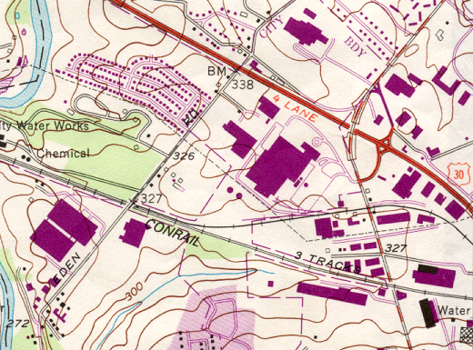
Manufacturing takes place in factories and industrial plants all across the country. Some regions of the country specialize in one or a few products. Small towns may have one factory that employs many of the locals, while larger cities, as we have seen, will definitely have large numbers of factories in multiple city locations. In between those extremes, small to medium-sized cities often have an industrial district in which a cluster of factories will be located. Factories are usually medium to large buildings, and are often collections of large buildings. On the older USGS quadrangles such as the portion of the Lancaster PA quadrangle shown below, the symbols for such buildings are either solid black or cross-hatched, showing the building's full size. Of course, on the newer quadrangles the only way to see such details is to activate the "Images" layer. Some facilities have unique characteristics, such as the many round tanks of an oil refinery.

As we have seen, transportation is a key consideration both for bringing in raw materials and for delivering the finished products. Roads and railroad spurs are often nearby. As mentioned above, in coastal towns and cities, industrial facilities may be located near shipping facilities, such as docks projecting from the coast or river's edge, or dredged channels in adjacent waterways.

Tertiary-Level Activities

The retail and services sector activities take place in commercial districts of cities, in the shopping and office complexes of the suburbs, and in a huge number of small establishments scattered around the countryside and around city neighborhoods. Retailing includes warehouses which may be located close to the manufacturers in cities, and are commonly moving to suburban and even rural locations along major highways. Services include banks, educational institutions, hospitals and many other related activities, and also government offices for everything from welfare services to research laboratories. These are the white-collar jobs of America, which have come to define middle-class living.

Some retail and service providers, such as shopping centers, schools, churches and hospitals, can easily be identified on USGS topographic maps. The USGS has made a point of representing them because it serves one of the roles its quadrangles are designed for: to serve as a way to identify major resources in a time of emergency. Schools, churches and hospitals would be vital in providing shelter, food distribution and restrooms for larger numbers of people.

In cases where map symbology does not label specific structures there are still ways to identify tertiary-level activity. If you are looking at an urban area shown by the dense concentration of large urban buildings on the Images layer, or by the urban tint on older quadrangles, it is very safe to presume that there are many retailers and many service jobs. No population concentration can survive without them.