The Basic Mapping Process
Cartographic Context
Topographic maps, such as the USGS quadrangles we are studying this semester, can be complex and detailed. The complexity of a topographic map invites the map user to spend time studying it and looking for details. Since a lot of different kinds of information are crammed in together, the cartographer has to pay attention to things like whether some features are covered by other features, and whether labels can be read easily.
Topographic maps can realistically be created using GIS programs, if you are willing to pay a lot of attention to the detail. In this unit we will talk about some of the principles of map design that can make more effective topographic maps.
The process to create a map consists of these four stages:
- Determine the map's purpose.
- Compile the map.
- Decide which layers to include: consider precision and accuracy.
- Decide the map's scale: determine its size and extent.
- Decide how to resolve distortion issues: determine the map projection.
- Decide on all map symbols.
- Decide which features need labels.
- Compose the map.
- Add all other information: statistical or textual (title, legend, etc.).
- Position all the above elements within the viewing page.
- Publish or present the map.
The Purpose is the most important stage, as everything else depends on it. What is the intended content? Who is it for? What knowledge of the map's content (such as locations and layer relevance) do you expect your intended audience to have? For projects in which we are drawing a map for public display (in a publication or online, for example), a critical part of the map's purpose is to make the map communicate.
Though it is being considered here in the context of topographic maps, the basic process applies to any type of map; topographic or thematic. The focus in the discussion below will be on map compilation, with map composition to be covered further along in this course.
Layer selection incorporates issues we have examined already, including sources, formats and attribute data. The related concepts of precision and accuracy are frequently covered in Math, Science and Social Science courses; they will be examined in depth later in our discussion of data-dependent thematic maps. The other discussion relevant to layer selection is the importance of understanding location and coordinate systems, both in general usage and in their GIS details; that will be examined in the next two units. Map scale and map projection will be considered in forthcoming units. Map scale obviously relates to the relative and absolute sizes of things on the map; the need for a map projection is due to the fact that the Earth is round, but the map sheet is flat. Topographic projects in which the goal is to depict accurate locations will emphasize those scale and projection decisions, so those will be important units to understand. Map symbols and labels will be demonstrated below, since they strongly impact that "communication" objective of all maps produced for a broader audience. Finally, publication is seen as the ultimate goal of most map projects.
Analyze the Process
Follow these Two Examples: The two scenarios shown here emphasize topographic mapping, one representing the area covered by a USGS quadrangle (about 50 to 65 square miles, depending on the latitude) and the other representing a map of the Millersville University campus (250 acres, or about 0.4 square miles). Both would be expected to show a lot more detail than a topographic map of Pennsylvania or the USA.
The first step is to determine the map's purpose.
| The USGS Topographic Quadrangle | A Millersville University Campus Map |
|---|---|
The purpose is to provide general descriptive information to a broad variety of users.Those users include field researchers in geography, geology and biology; campers and hikers; local governments who lack their own mapping agencies or resources. Measurement standards for locations and sizes of features were high. The symbols to be used were to be as obvious as possible so that a legend on the map would not be necessary. |
We could choose a broad variety of users, as the USGS did, but instead let's decide to make a map aimed at guiding campus visitors to on-campus sporting events.We need roads, parking lots, buildings and athletic fields. The measurement standards for locations and sizes don't need to be very high since the map covers a small area. The map should be oriented with north at the top so that it corresponds to any other map the visitor might use to get to the town of Millersville. |
The next step is to select the map's layers.
| The USGS Topographic Quadrangle | A Millersville University Campus Map |
|---|---|
Because the USGS quadrangle must serve so many purposes, they had to include a huge variety of map layers.Recall our tour of the layers displayed in the layers list for a modern digital quadrangle in Adobe Reader. It included physical landscape elements and cultural elements. The newer maps do not contain nearly as many different types of information as the older ones did. A guide to virtually all symbols used in the paper maps printed before about 2000 is below on this page; each symbol shape or group of symbols with related shapes or colors can generally be interpreted as representing a different map layer. |
The campus map has several necessary layers representing the most prominent features of campusBuildings, roads, parking lots and sidewalks are obviously on that list. The source for the roads, buildings and property lines within Lancaster County, PA is the Lancaster County government, though the level of completeness and detail from a group responsible for the entire county may not suit some of our needs on this campus map. Then, given our purpose of focusing on sports-related campus locations, we need to set up some of those layers as point features (entrances to stadiums, fields and gyms), line features (cross country runners' route) or areas (buildings, athletic fields and designated parking lots). We could use county or other sources of layers to act as a basemap (a background map), though, so that Millersville University does not appear to be an island surrounded by nothingness. |
Next, decide the map's scale.
| The USGS Topographic Quadrangle | A Millersville University Campus Map |
|---|---|
The USGS produces a range of topographic maps at different scales. At the scale that will be used most frequently in this course, one inch represents 2,000 feet.These maps cover 7.5 minutes of latitude and 7.5 minutes of longitude. The paper size is not one standard dimension, because 7.5 minutes of longitude in southern Florida is much wider than 7.5 minutes of longitude in Maine. The map scale is a consideration of both the size of paper to be used to print the map, and the amount of detail to be shown on the map. This standard map series is the most detailed they produce, and there are nearly 54,000 different maps covering the United States in this series (Thompson, p. 108). |
To make the campus map easy and cheaper to print and distribute, we can print it on 8.5 inch x 11 inch paper.The size and shape of the campus best fits the paper held horizontally (landscape mode). Those dimensions are the primary determinants of the map scale. In this case, as with standard maps of the United States, we need to fit (all of) an irregular shape onto a rectangular paper area. As often happens in these cases, the map scale is not a nice round number unless we shrink the map or change the margins, or get lucky. |
The next step, determining the map projection and how the latitude-longitude grid should be represented, is generally less of an issue at larger scales like the ones we are developing.
The next couple steps involve deciding the symbols to display each layer and which layer(s) need labels within the map to identify specific layer features.
| The USGS Topographic Quadrangle | A Millersville University Campus Map |
|---|---|
The USGS has their standardized collection of symbols for its 7.5-minute series topographic maps, which are available for viewing below. Labeling is similarly based in their established procedures.The symbols have evolved over the years and vary slightly between the 7.5-minute series and their maps at other scales. However, the fact that they have been a reliable source of information for a long time makes their symbol choices worthy of respect.General user familiarity with the USGS quadrangles' symbology also stems from the fact that their symbols are designed to be as natural as possible. Choosing colors and symbol shapes that are least likely to be misinterpreted results from those years of experience. USGS maps, as "public domain" publications, are the base maps used by several publishers of county road atlases and by local government agencies for a variety of their maps. Their names for places and natural features are considered authoritative. The USGS also has developed label positioning strategies that are very effective. With so many revisions of every quadrangle over the decades, every imperfection has likely been resolved. |
Since our campus map's purpose is so narrow, the necessary labels will likely be obvious.The venues and surrounding buildings, the roads and parking lots closest to those venues, and any other locations we always want visitors to be aware of will likely make our list. |
The addition of text outside the map is intended to enhance the map content.
| The USGS Topographic Quadrangle | A Millersville University Campus Map |
|---|---|
USGS quadrangles include a great deal of technical information, both within the map area itself and especially in the margins of the map.Again, the USGS topographic quadrangle is designed to be of high technical quality, and standardized on a particular map scale and latitude-longitude grid for its 7.5-minute series topographic maps. The information presented in the map's margins ranges from the names of the responsible agencies, to the map's title, publication date and scale, to the details of how and when certain components of the map (such as the aerial photography and field checking) were accomplished. One of the goals of this course is that you are able to examine all of the text information presented on topographic quadrangles and explain its meaning and significance. |
The first step, deciding the purpose of this map, goes a long way toward determining its text content.Since we decided that this map should guide campus visitors to on-campus sporting events, the names of roads, sports venues and key landmarks such as major buildings should be shown. The map's title and legend will also help to ensure that its purpose is met. Finally, all maps should have a date stated somewhere, so that users can always know whether the map is current or out of date. |
Cartographic Compilation
What is Cartography?
Cartography is the art and science of making maps. It requires an understanding of map reading and map analysis as ways that users will take in the information contained in a map, so that the cartographer is able to present the information in the most effective way. Consider that to be a potential direction you could follow after learning the skills you will acquire in this course.
GIS is necessary for Cartography, but not vice versa. This means that you are gaining a new skill when you add Cartography to your other GIS skills. GIS software is not optimized for Cartography. Many, if not most, defaults are cartographically poor choices, and many cartographic elements of ArcGIS do not reflect the ways cartographers work. Remember, ArcGIS is a computer programmer's translation or interpretation of how to make maps, and is very focused on spatial analysis. However, ArcGIS today has much better cartographic capabilities than it did 5-10 years ago. It also provides ways to over-ride the automatically-generated defaults so they can be executed "manually." You will get a taste of those customizations in this course but most of that will require further coursework in GIS and cartography.
Compilation is...
Compilation is essentially the collection of information for the map project. As noted above, it includes deciding which layers to use and what attribute data they must include. Compilation also includes symbolization decisions (see below) and the addition of any titles, labels or other text on the map.
Keep in mind that early hand-drawn maps did not follow the "layers" concept that now forms the foundation of GIS software. There was certainly the concept of "many kinds of information" but it was often driven as much by what could be achieved from an art and design perspective: maximize the amount of information while retaining readability. The cartographer was selective about what was necessary to include in the map. If a smaller road was in the way of a label for something important, the road was removed. Computer technology does not allow for that level of flexibility without expending extra effort.
Topographic Map Symbology
The Symbols
Symbols hold the meaning of every map. Later in this course you will learn that you can use detailed topographic maps with their abundance of symbols to glean evidence of the map area's physical and cultural landscape histories. In that context, it will be important to understand the association between symbols and their meaning.
Symbology choices involve all characteristics of each symbol, including shape, color(s) and size. Fortunately, there are lots of examples to follow these days, with maps so readily available online. Pay particular attention to the USGS quadrangles we will use. The next major topic below will demonstrate some of those choices in ArcGIS.
You will be using USGS topographic maps for interpreting several different aspects of our surroundings in later portions of this course, and you will notice that the USGS maps have hardly any legend and provide only minimal explanation of the meanings of the colors and other symbols on the map itself. Part of what enables their maps to be effective, despite that lack of legend, is that they have chosen colors and symbols which can be easily, almost intuitively, associated with the actual feature.
USGS Topographic Symbology
However, it turns out that there is a legend included with the newest digital USGS quadrangles. To access the legend, look in the same group of icons to the left of the map in Adobe Reader where we opened the list of map layers. Just above that is a paper clip icon which, when you hover a mouse over it, displays a message saying "Attachments." It means that within the PDF file containing the map is another PDF file containing the legend document. The document is named "US Topo Map Symbols.pdf" and a double-click on its link opens it as a second tab within the Adobe Reader window. The first page of it is a rather elaborate title page, and at the current writing there is only about a page and a half of actual symbols and their meanings. They provide very little additional explanation of the symbol, beyond their name for what it represents. So be prepared to look up some of the terminology if it is not already familiar to you. Of course, you can also ask questions.
The table below represents a guide to all of the symbols used on the traditional paper versions of USGS topographic quadrangles. Examine it for its variety, and for the way the nature of each symbol resembles the map feature it represents. Even though many symbols have changed slightly in the newer digital versions of the USGS quadrangles, that resemblance is still maintained. In their current implementation the quadrangles are not displaying the same variety as shown on the older quadrangles, but the potential is certainly there for that level of detail to return.
The legend graphics that the links below will reveal are from an older USGS symbology brochure (USGS). Compared to the current legend document described above, that brochure consisted of a title page and three pages of symbols. Having so many more symbols back then, the categories were a little more helpful in providing context, but you still might need to look up some terminology. At this stage of the course, you are not being asked to learn these symbols; however, later in the course you can come back to this topic to help you navigate the USGS quadrangles. At this point the key is to notice the variety and ease of understanding most of the symbols.
| Physical Landscape | Human Landscape |
|---|---|
| Contours | Boundaries |
| Contours - Topographic and Bathymetric | Boundaries |
| Control Data and Monuments | Land Surveys |
| Projections and Grids | |
| Land Surface | |
| Surface Features | Transportation |
| Mines and Caves | Roads and Related Features |
| Rivers, Lakes and Canals | |
| Vegetation | Railroads and Related Features |
| Vegetation | Transmission Lines and Pipelines |
| Submerged Areas and Bogs | |
| Buildings | |
| Water | Buildings and Related Features |
| Rivers, Lakes and Canals | |
| Marine Shorelines | |
| Coastal Features | |
| Bathymetric Features | |
| Glaciers and Permanent Snowfields |
An Alternative Example
Topographic mapping works best if the symbols and colors are visually suggestive of the feature they represent. USGS symbology is so standard and recognizable that it is easiest to stick to its conventions. Blue for water, green for vegetation and brown for ground features all emphasize natural color associations.
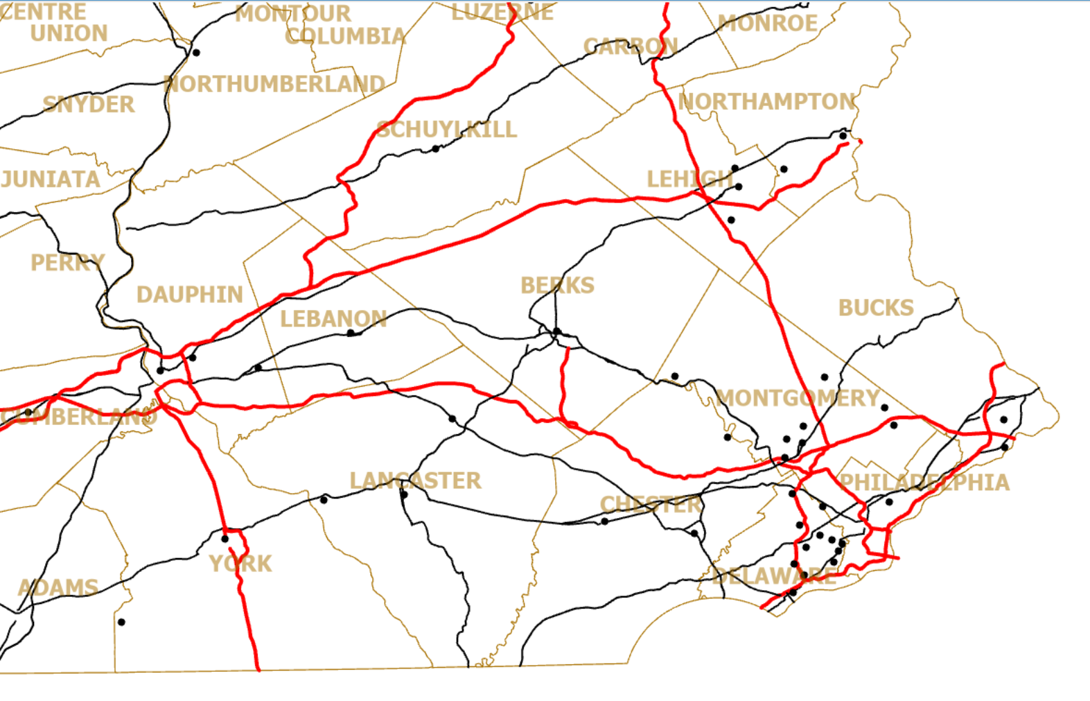
Since black, red and purple are not common in nature, it is easy and obvious to associate those colors with human (non-natural) features such as roads, urban areas and photorevisions. For example, Pennsylvania Department of Transportation highway maps, like the examples below (PA Dept. of Transportation), use orange to represent cities and yellow to represent the suburbs surrounding those cities. On the other hand, they also use green and blue to represent certain highways, which is an odd choice.
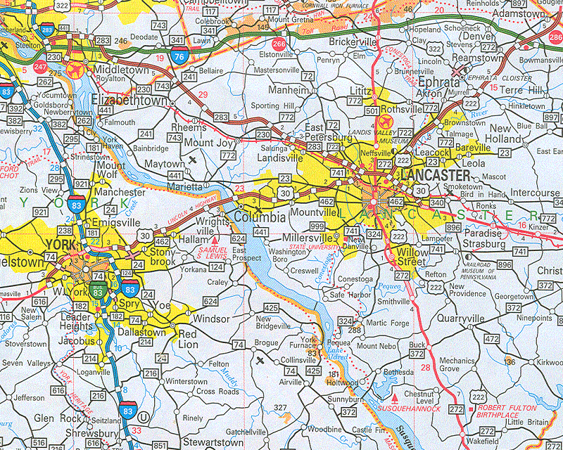
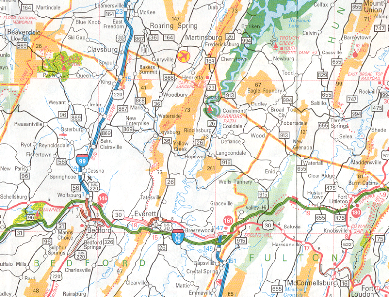
The Symbol Colors
Symbol colors for areas will tend to be pale colors so that text placed within the areas is still legible. One challenge is that there are only so many such pale colors that are easily distinguished. The same orange used on the Pennsylvania highway maps to represent cities, is also used to represent State Game Lands, which are always located in rural areas. The subtle difference of the cities being surrounded by a dashed black outline, while the State Game Lands have no outline but do feature their identification number, reinforces the idea that topographic maps are meant to be studied carefully. The rural area depicted in the second part of the same highway map (PA Dept. of Transportation) below shows two different shades of solid green plus a mottled geen-and-yellow pattern to show additional areas. The darker green is for federally-owned land within Pennsylvania, the lighter green is for Pennsylvania State Forests, and the geen-and-yellow pattern represents Pennsylvania State Parks.
Symbol colors for point locations and line features, such as towns and roads on the highway map will tend to be darker so that they are clear in spite of the small amount of paper they occupy. See how many different symbols you can identify on this map sample, and whether you can infer the purpose of each one.
Topographic Map Labels
Labels are an important aspect of the information content of maps. At the level at which we are starting here, I recommend keeping the use of labels to a minimum, perhaps just for one or two layers of area features. The layer's labels are related to the location of the layer features, but have their own locations. In a very cluttered or complex map, thought, overlap might be unavoidable, and the best solution might be to remove a layer's labels.
Text on Topographic Maps
Text size (for there should be lots of labels) has to be large enough to be read, but small enough not to distract from the map information. Because topographic maps are meant to be studied, text sizes can be very small indeed. It is as if the cartographers expect map users to have a magnifying glass available.
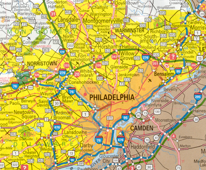
Another thing that you will notice about text on published topographic maps is that the cartographers have to be selective. They have to weigh the importance of a particular name's presence on the map against its effect on making the map too cluttered and confusing. Areas that are more developed, with more roads, towns and other significant places, will have less significant items (for example a popular local park) eliminated from the map, while areas that are very rural will include even very minor details (like a park that hardly anybody uses).
The map below, taken from the same larger paper map shown above, (PA Dept. of Transportation ) illustrates that contrast. Anyone from the Philadelphia suburbs will complain that the first map excludes many familiar names of local towns, many with populations in the thousands. To make up for that shortcoming, the Pennsylvania Department of Transportation highway map that it was excerpted from has an enlargement of Philadelphia on the reverse side of the map. The second map of a more rural area in central Pennsylvania contains many small towns whose total populations are in the hundreds, smaller than a few blocks of those missing Philadelphia-area towns, and even with that there are areas with no symbols or text.
One of the best practices for cartographic work is to create a list of text conventions you will follow on a particular map project. Each different type of map information (layer) should be labeled with its own combination of text size, font, italics and other text characteristics. That way, if you make effective choices,the text can be made to work with the symbols to help differentiate map features.
Topographic Symbols and Labels in ArcGIS
Symbology in ArcGIS
The Layers
The Contents panel in the ArcGIS Pro window gives you the ability to determine the order in which the layers are drawn. Remember the "layer cake" analogy. Think of the layers in the Contents list as being able to cover the layers below it. If a layer of point features is higher in the list than a layer of area features, the points will be visible, but if the layer of areas is above the layer of points, then the points will be covered by the areas and the points will not be visible. Simply click (to select) one layer and then drag that layer higher or lower in the Contents list.
You may have already noticed that each layer in the Contents list also has a checkbox to the left of its layer name. That means that each layer can also be turned off and on in the course of an ArcGIS session. That may also help when making symbology decisions. Consider this: any layer can be added multiple times in the same map project. If you have several ideas for different symbols or symbol characteristics, add the layer once for each idea and then turn each alternative version of that layer off or on in order to make your decision.
The Single Symbol
The initial symbology for each new layer added to a map is termed "Single Symbol" symbology. This means that every feature in that layer is drawn with the same symbol style, color, and size. The symbol type depends on whether the layer contains points, lines, or areas. Each feature category has a default symbol type. The default point symbol is a circular dot of a small size, a random color, and a thin black outline. The default line symbol is a solid line of a narrow thickness and random color. The default area symbol has a random color and a thin medium-gray outline. For some map layers the single symbol might be all you need. It is likely, though, that the default symbol is a poor choice, so our first task is to learn how to change the defaults.
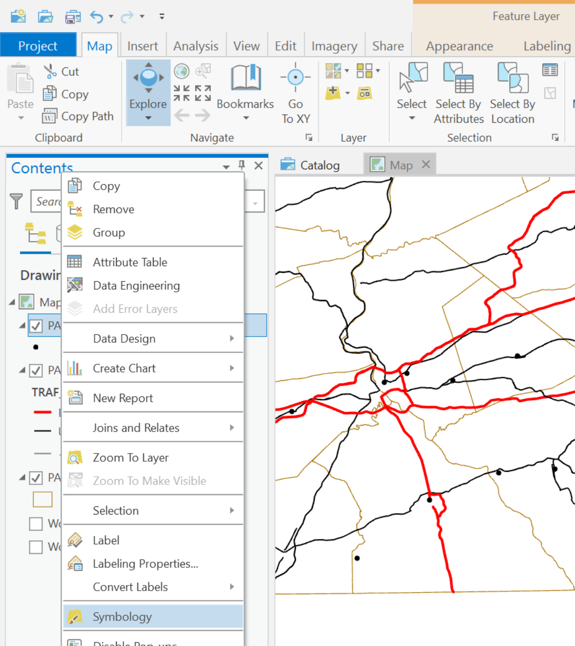
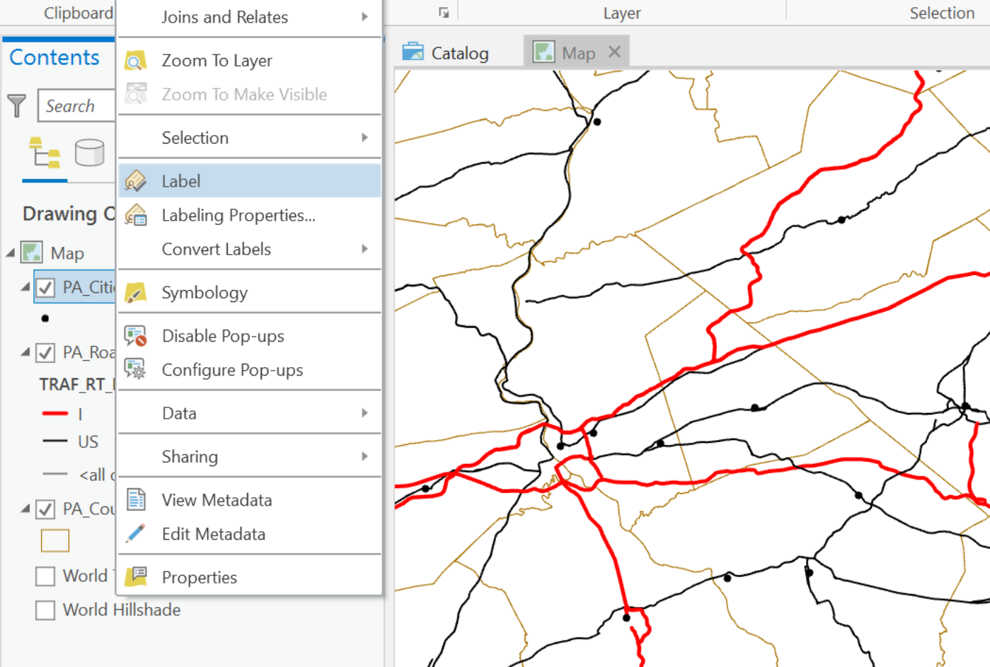
Generally, the symbol change procedure starts with selecting that layer in the Contents list. Then, right-click the layer name and a menu will open. Select the "Symbology" menu option. The Symbology dialog panel will open from the right side of the window. It is also possible to open this dialog directly from the Contents list by clicking not on the layer name but directly on the current symbol itself. [Note: there are other ways to open the symbology dialog panel but explaining only these will keep the process simpler here.]
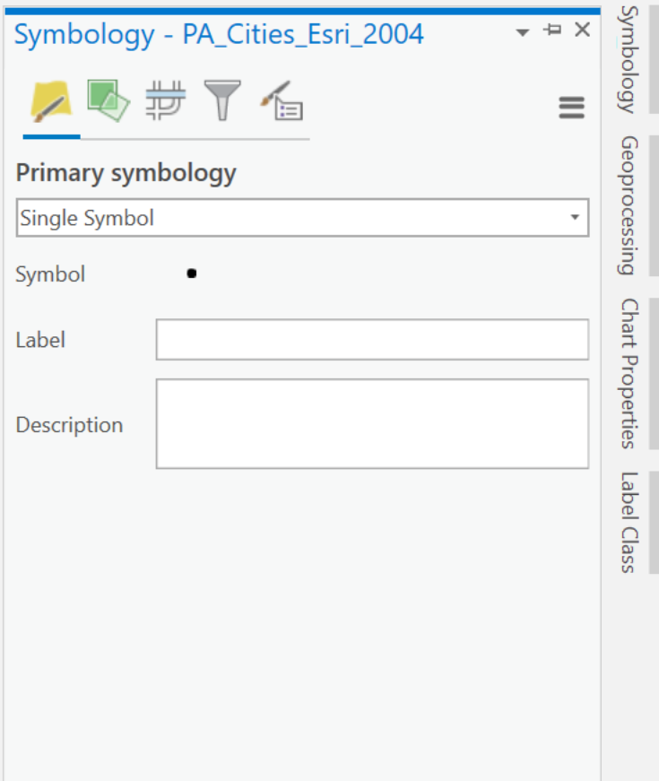
The appearance of the Symbology dialog panel will vary with the type of feature (point vs. line vs. area) and the type(s) of symbol(s) chosen. The example below shows a very simple symbol for a points layer. Notice that two boxes for "Label" and "Description" are empty. The Label box will contain text in some situations and that text will appear to the right of the symbol(s) in the Contents list. When the box is empty, as in this image, you can type your own, and you can always edit any text put there in other ways. This will be useful later when you learn to construct a legend for the map.
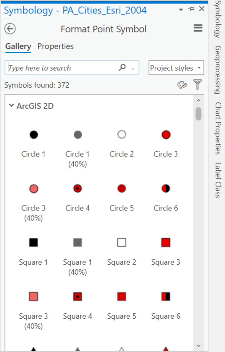
To change the symbol, simply click on the symbol that is there and the dialog view will switch to a collection of many symbol choices. No matter which type of features you are working on, a large variety of symbol options will be available. The point symbols in our current example can vary in shape, size and color. Edge lines, or outlines, are an option, with the outlines potentially having different colors and even thicknesses. With the point symbols only, you can also elect to change the angle at which the symbol is drawn, turning a square into a diamond for example (this does not pertain to line and area symbols). The dialog box shown below can be scrolled down to reveal many more choices, some of which are generic shapes like those shown and many of which are picture symbols depicting airplanes, gas pumps, trees, and many other options. The generic symbols shown will have a limited choice of colors, but once you have chosen the shape you prefer you can click on the word Properties below the dialog box title and choose from several aspects of the symbol to change. For example, for the point symbol you can change the symbol color and size.
Since you are relatively new at this process, the safest approach is to choose any of the picture symbols or to choose a very simple generic symbol and change only the most basic properties. If you have goals of making more elaborate, complex or subtle design choices, you should know that ArcGIS Pro can probably accommodate them. However, that is beyond our scope here.
Be aware also that the symbology choices change for line and area feature types. Line symbols have the greatest similarities to point symbols. Again, there are more generic line styles as well as more complex designs labeled for specific situations. Area features tend to be a bit more complicated because it is less likely that you will cover a map with areas that are all the same color. [Note: symbolizing a layer with areas of varying colors would make it a thematic map, which will be a focus much later in the course.] It is also possible to make the fill color of the areas transparent while keeping an outline, as you have seen in the previous examples with the Pennsylvania counties layer; it is much more likely that you will alter the outline characteristics (that process looks same as the choices for line symbols).
Symbology Based on Unique Data Values
Symbology can also be based on attribute data stored in the map layer's shapefile. We examined attribute data in the previous unit of this text and will explore it in much greater detail in the later units on thematic maps. The capability we are after here depends on having a data column in which there are several different repeated values. Most often the values are text, though this technique will work if the values are numbers, too. These repeated values can represent categories of the map features. Unique Values symbology creates a unique symbol (within reason) for each category of a GIS layer.
We know that a GIS layer is a collection of features in which all are the same type: points, lines, or areas. For example, a map layer of Pennsylvania cities might contain all 57 cities represented with black dots on the map, suiting a more topographic map purpose. Another way to symbolize the cities is to group them into categories based on values in one of the attribute table fields, such as whether the city is the location of its county's government offices: Yes or No. Each category could be represented by a different color of the same symbol, or by a differently shaped symbol. It is also possible to create the categories based on an attribute table field containing numerical data. However, quantity-based unique values require other considerations and will be examined later in this course as thematic maps. The current discussion will be based on categories derived from text values only, which are more likely to be used in topographic maps; however, the symbology distinction between topographic and thematic maps is not always clear.
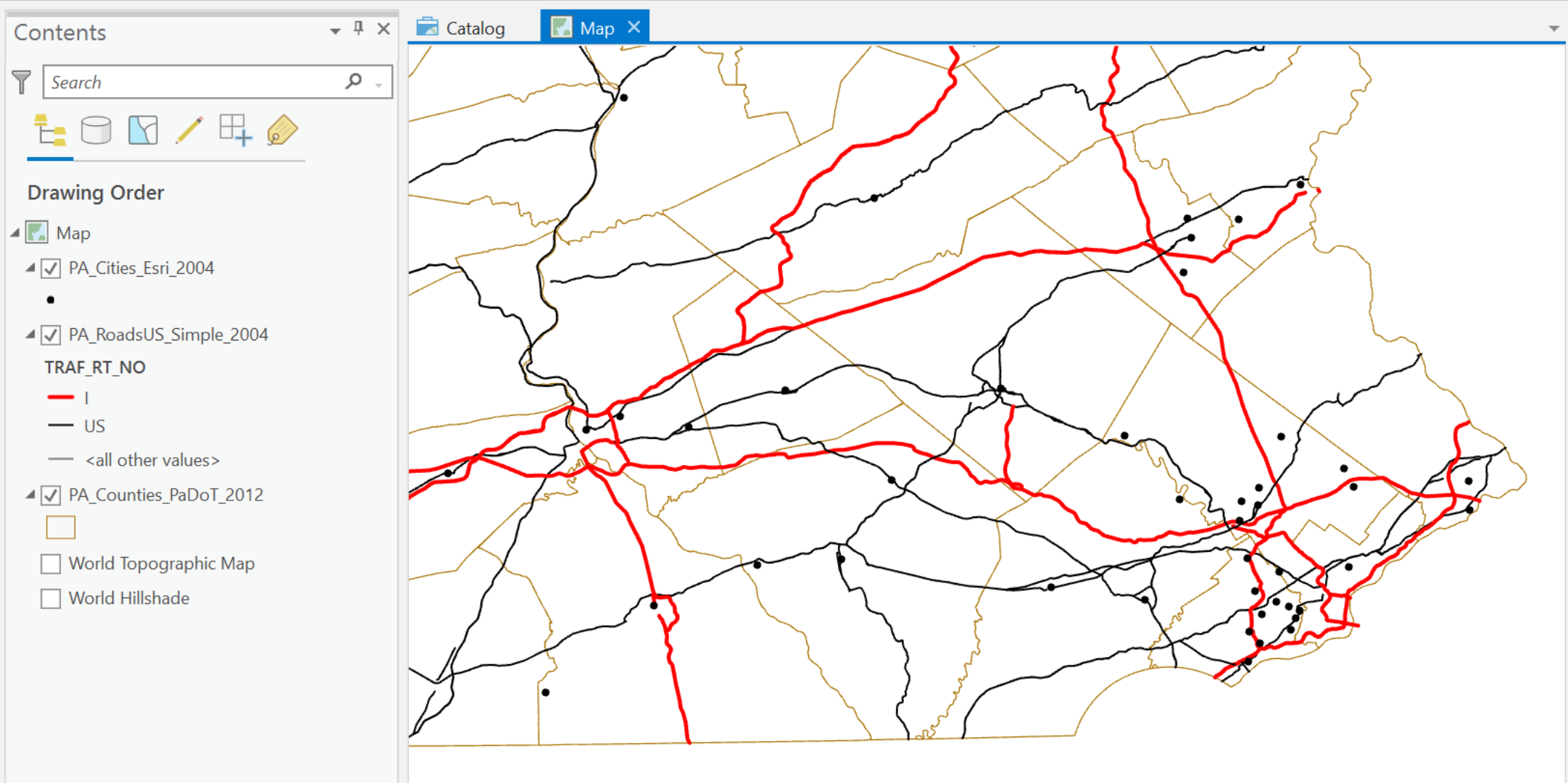
Allowing different symbols to represent the categories of features in a layer is referred to as "Unique Values" symbology. For our example, we will use the line features in the Pennsylvania highways layer (PA_RoadsUS_Simple_2004) on our map; the highways are line features, of course, and each highway has a name and a route number among other identifying characteristics. In road layers there are often way more features in the layer than you might expect to see. Each "feature" is a relatively short segment of road, usually from one intersection with another road to the next.
We start by opening the attribute table to ensure that a field containing the appropriate text exists. While there, take note of the name of that field. In the example we will follow, that field is "TRAF_RT_NO." It contains values that identify the type of highway in terms of which federal government program funded its construction and maintenance. The layer was constructed in such a way that only two different values are present. "I" represents highways that are part of the Interstate Highway System and "US" represents older highways built as part of the US Highway System. Both systems, which are very interconnected today, include most of the largest highways in the state.
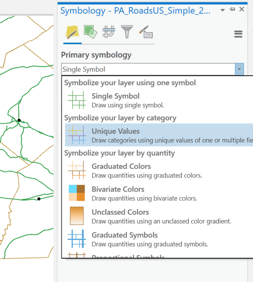
As noted above, the initial default symbology for the highways layer was a Single Symbol, a simple colored line. To change that option, open the Symbology dialog and click on the box just below the label "Primary Symbology." As shown below, in the menu list that opens, scroll down and click on the "Unique values" option.
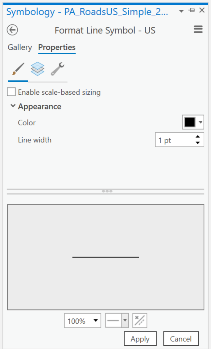
Initially, no value field is identified so the next step is to identify it: the "TRAF_RT_NO" field identified above. Once the field is specified, all the specific category values from that field are added in the list below, and next to each one is a corresponding default symbol. As happens when a layer is initially added, the default symbols are simple shapes (lines in this case) randomly colored. A single click on each of the default symbols will open the same Symbology dialog used earlier, to either its Gallery view or Properties view; of course, this time its purpose is for selecting line symbols to replace the defaults. As you select each separate category's symbol you will have to click on a button at the bottom of the dialog box to Apply the symbology choice.
Close the Symbology dialog by clicking back on the map (you will be prompted if any of the symbol choices have not been applied). Notice (see the map below) that the highways layer has been modified, and that its listing in the Contents list now shows both new symbols, each labelled with its text data value, along with a symbol (a default that was not changed) to represent any roads in the layer that had neither the I nor the US data value. If at any point you are unhappy with the symbol chosen for any specific value, you can click directly on that symbol in the Contents area to re-open the Symbology dialog.
Labels in ArcGIS
Labels in ArcGIS Pro
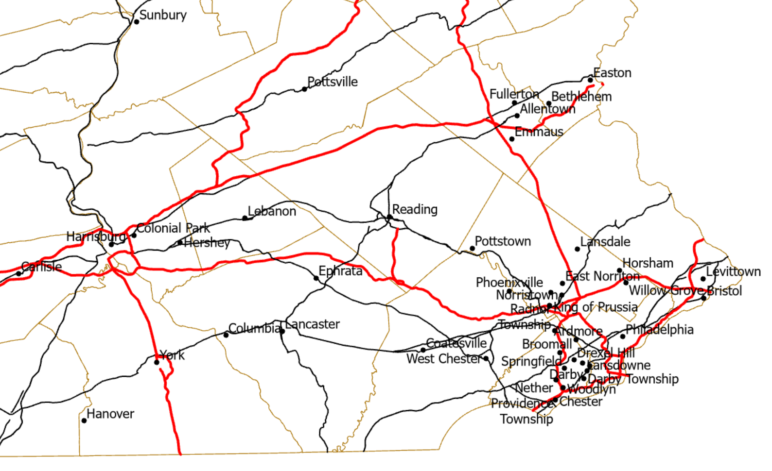
Consider the ArcGIS map below to be a GIS "work in progress." The cartographer using ArcGIS Pro decides that the spatial context will be enhanced by including labels and decides to label the cities in the map. The labels are added by right-clicking on the layer's name in the Contents list and selecting "Label" from the menu that drops down (shown below).
The next map below shows the results of the labeling. By default, ArcGIS Pro looks for a data field (column) in the Attribute Table whose name includes "name" in some form and uses that name. Labeling the cities turns out to be a poor decision because so many of the point locations were close together. If you look very carefully, ArcGIS even made it difficult to tell which label was attached to which point, especially near Philadelphia.
There are potential solutions for such an awkward label arrangement, but most require altering the attribute data or using other advanced tools in ArcGIS. Additionally, if a data field with appropriate names was not selected by default, it is possible to change the label field. Both these tasks will begin with right-clicking on the same layer's name and selecting "Labeling Properties" (just below the Label menu option). Unfortunately, the dialog box that opens is much more complicated than the others we have viewed so far, so if the default labeling is not effective, at this level it is safer to try a different strategy. For example, if the city names are not necessary, one strategy would be to add labels for the counties layer instead. For the next map, the cartographer turned off the labels by selecting the Label menu option again from the layer's right-click menu and then turned on labels for the counties layer. Initially, it is not much better.
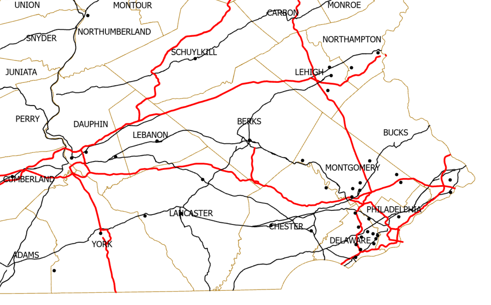
The default label style, with small black lettering does not naturally communicate as the name of a large area and the labels interfere with the black roads and black city dots. To solve these problems, the cartographer decides on a larger, bolder label in a lighter color to help the county labels fit better with the map symbols. Unfortunately, the path to control the label fonts and other details of the labels is just as complicated as the other labeling properties, but it is important to note that it is possible to change these elements, as shown below.
The resulting map (below) is much less cluttered. This example is not yet perfect, by any means; for example, notice that ArcGIS Pro was forced to include the labels for many northern counties just because tiny corners of their area were within the map. However, the goal of giving some geographic context for the map was accomplished.
Basemaps and Aerial Imagery: Raster GIS
Basemaps
What is a Basemap?
As described above, it is possible to create your own topographic map, and doing so is an excellent way to build your GIS skills. The biggest advantage of doing so is the fact that you customize it to your needs. The work involved can be significant, though, since it involves collecting multiple layers and symbolizing each one.
There are situations where the topographic map that you can create cannot meet your needs (for example, if some layers are not available), or would take too long to put together. For those situations ArcGIS allows you to add a basemap. The basemap is added as one or two predesigned GIS layers that display a variety of types of information. Basemaps are published as imagery, or raster, layers (see the discussion and examples below), making them easier to manage, but impossible to alter. In all the basemap layers described below you will see the content change if you zoom in or out on your map by a significant amount.
Currently the number of basemaps available in ArcGIS is 28, but that is subject to change. Here are a few general types of basemaps you will see:
- Imagery, with or without labels: satellite images and aerial photography (read more about these types of GIS data below).
- Topographic maps of different styles, with or without labels. Different topographic basemaps represent the symbology styles of different conventional map publishers.
- "Canvas" basemaps, with or without labels. These provide simplified symbology and muted colors.
- Terrain representations, with or without labels. These basemaps emphasize the physical landscape.
- Other styles, some of which are more specialized.
Even though each basemap option is added as a single selection in the dialog described below, quite a few of the options actually add two layers to your map: most commonly, one layer of symbology and a separate layer of labels. The advantage of this arrangement is that you can turn off one part of the basemap layer without turning off the other such as keeping the basemap symbology but turning off the labels. The basemap symbology layer will be added at the bottom of the Contents so all your other layers draw on top of it. The labels mentioned above in the list are sometimes an integral part of the basemap and other times included as a separate layer with its own checkbox. Often, the labels layer of the basemap will show up in the Contents list at the top of the stack, so the labels are always visible.
Procedure for Adding a Basemap
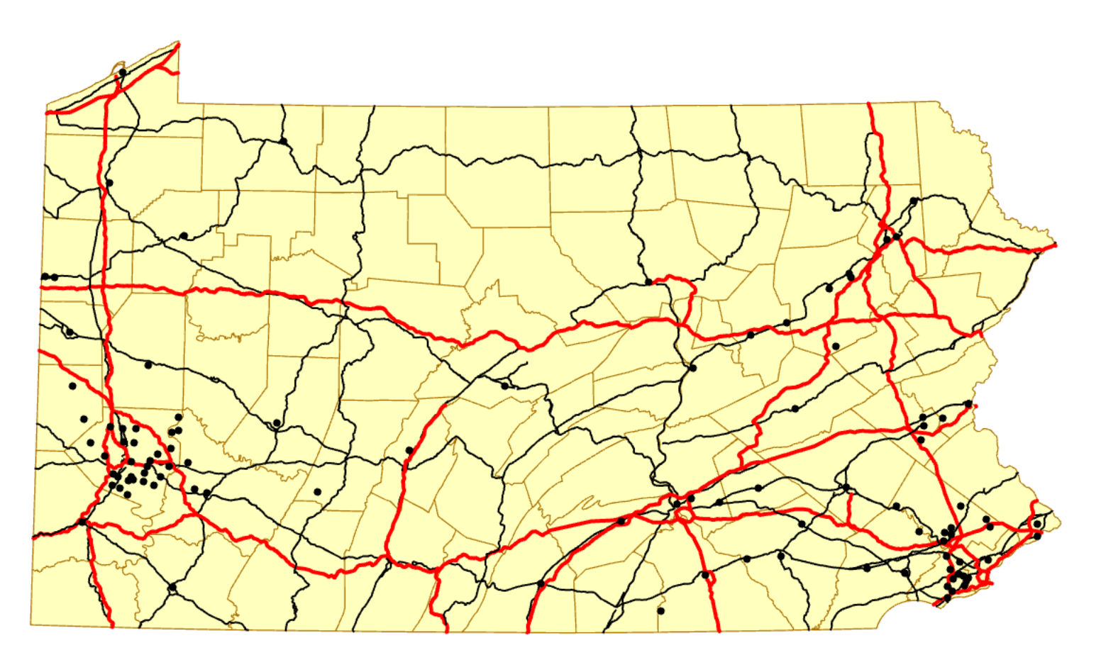
First, consider the map below. It may serve a significant purpose for a project showing the spatial relationships between cities counties and major highways in Pennsylvania. However, Pennsylvania is left "floating in space," as it were, providing no context about where there might be similar cities or highways in neighboring states.
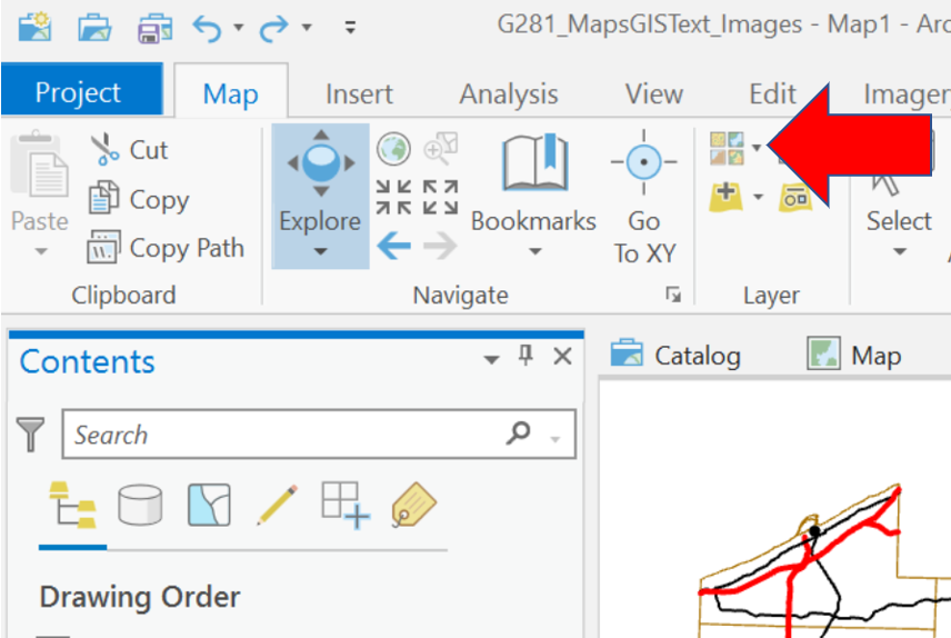
A basemap enables us to add that context. The command button to add a basemap is on the same ribbon menu and in the same section of that menu as the "Add Data" button used to add layers onto the map. Hovering over the tool icons there will enable you to see which one initiates the Add a Basemap dialog.
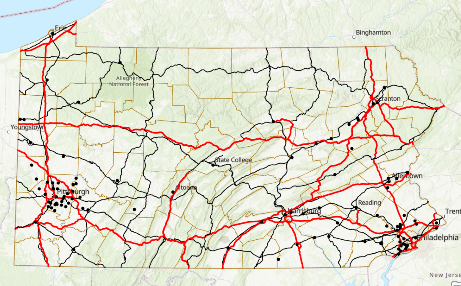
The menu that opens allows you to select from a number of alternative basemaps which are both named and displayed as samples, as described above. For our example, a general topographic map with more muted colors that allows our layers to stand out makes the most sense.
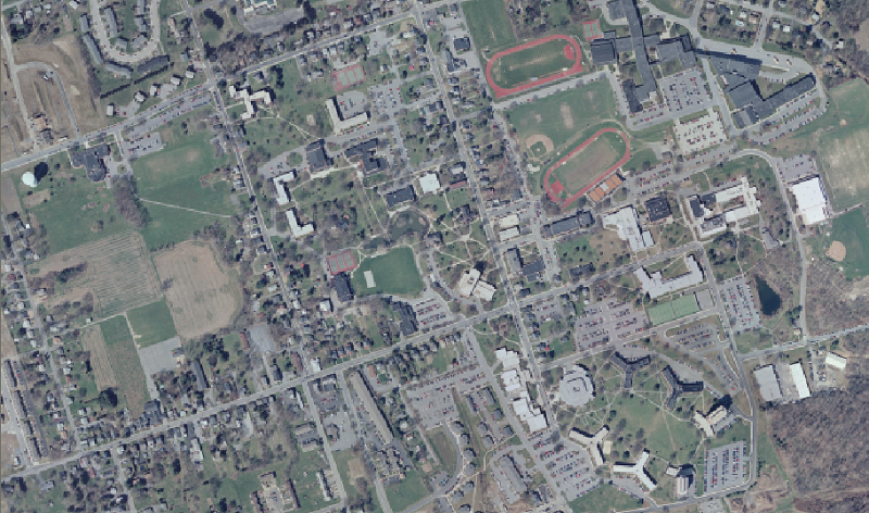
Aerial Photographs and Satellite Images
Aerial photographs (or air photos) are photos taken from airplanes and, increasingly, drones. Satellite images are taken From much higher altitudes above the Earth (thousands of miles) using digital imaging, also known as scanner, technology.
The first air photos were taken well over 100 years ago with early cameras using photographic film, but now they are increasingly recorded, like satellite images, digitally. Both technologies record the scene below them passively (without modifying the information recorded). That is the key difference between them and traditional "drawn" maps, but in most other ways, and in this course, they are considered to be maps. As a matter of fact, both image technologies are often used as the base information for creating maps, especially when GIS technology is used in creating the maps.
Aerial Photography
The Technology
In most sources now both film photos and scanned images are referred to as imagery or images. In the context of this discussion, however, to tell them apart, photographs will refer to images recorded on film. Photographic film is a technology that originated in the 1800s but proved very effective as a means for creating and storing a record of the Earth's surface below the airplane or other camera "platform."
The film is coated with chemicals, which are the real technology behind photography. The chemicals are light sensitive, which means that they change at the molecular level in response to being exposed to visible light. Visible light is the light that the human eye is sensitive to, the form of light that illuminates our surroundings. Black and white images were the most common means of capturing these images, because the light-sensitive chemical used to record the shades of gray can record a finer (more detailed) image.
The other key photographic technology, still part of modern digital imaging technology, is the camera itself, especially its lens. Aerial photography cameras are larger than personal cameras, and their lenses are much larger, too. In fact, instead of the 35 mm film (that measures the film's width) that has long been standard for personal photography, aerial photographs are recorded on 9 inch wide film.
Aerial photography has become so specialized that, in addition to using specialized cameras, the firms that do this work also employ specialized airplanes, with windows in their bellies for multiple cameras, each of which is mounted on gyroscopes to keep the cameras level. The cameras are able to take photo after photo (not movies) of the scene below, in such a way that each photo overlaps the previous one by about 60 percent. The plane flies a carefully planned flight path that also ensures that each parallel row of photographs overlaps the previous row, and no part of the scene is missed.
The Processing
After the coated film has been exposed during the flight, it must be developed, and then printed. Developing generally produces a film negative. In the printing process, light is passed through the negative to fix the light sensitive black dye on the print paper. The resulting print is a faithful record of that landscape, in shades of gray, from white to black.
Again depending on the lenses used, the print paper can range in size from smaller than the 9 inch wide film to three to four feet wide. As with many mapping technologies, the military played a significant role in helping to refine the technologies and processing needed to produce high-quality aerial photographs.
Color in Photographs and Images
The Visible Spectrum
Black and white photographs, we said, portray the landscape by dying the print paper with white-to-gray-to-black ink according to how much light the film negative lets through. The brightness is measured in general from across the entire visible light spectrum.
Color photographs use the same technique, with two minor exceptions: First, the color photography film is coated with three different light-sensitive chemicals. Second, each of those three chemicals is sensitive to a different but narrower part of the same visible light spectrum.
Which colors are recorded by the three film chemicals? The selection is based on another color representation you have most likely been taught: the color sequence known as "ROYGBIV."
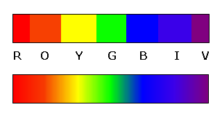
The Processing
Three colors out of that sequence, generally the primary colors RGB (red, green and blue), are used to describe the different chemicals. It is not only those specific colors that are recorded, though; each chemical is sensitive to about one third of the spectrum centered around those colors. But, all of those colors can be stored as a combination of different proportions of red, green and blue.
The printing process for color photos also triples the processing steps. In the development process, each chemical layer has its recorded proportion of light penetration fixed. In the printing process, each color is added as ink of the same color in those proportions to make the color photographic print. When we look at the complete color print, those three inks combine to form every color, with complete saturation with all three colors yielding black.
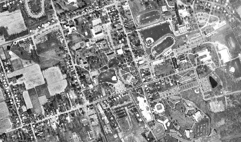
False-Color Aerial Photography
The electromagnetic spectrum continues outside of the visible light spectrum. We cannot see any light in that part of the spectrum, but it is there nonetheless. Ultraviolet light (just beyond the Violet end of the visible spectrum) does not generally provide significant information. Infrared light, on the other hand, can reveal a great deal about waste heat in urban areas and about plant health in agricultural and natural areas. The infrared light energy can be recorded by the same approach of finding a chemical coating that is sensitive to exposure to just that part of the spectrum.
The invisible nature of the infrared light complicates the printing process for color photos. Since there is no such thing as infrared dye, the printing process for these photographs continues to use the three conventional inks, red, green and blue. As with conventional color photography, these inks are used to print the three chemical layers on the film; in order to accommodate the infrared layer, the blue layer is eliminated. Each chemical layer has its record of light saturation fixed, and then the green layer is printed using blue ink, the red layer is printed using green ink, and the infrared layer is printed using red ink. Again, when we look at the complete color print, those three inks combine to form every color, with complete saturation with all three colors yielding black. Now, however, areas of the photograph that are dominated by red colors are areas rich in infrared energy.
The webpage linked here provides another explanation of this technology, and also displays several sample color-infrared air photos (GeoMart).

Images Based on Scanner Technology
Modern photography is almost entirely digital, completely different from film photography.
The medium today is not film spread with chemicals, but sensors tuned to detect and record a narrow beam of light. Printing photographs, when it is necessary (since we can readily recall and display images on a variety of digital devices), is not done with light-sensitive processing but with pinpoint control of tiny dots of ink. In other words, the basis of modern technology is devices that divide the scene and the page into ever-smaller parts, referred to as pixels.
Digital photography has followed a similar development path to that of film technology in the sense that it started out black and white before developing the ability to produce colors. Black and white display technology emerged before color on devices from televisions and computer monitors to cell phone and digital camera viewing screens. In black and white devices, each pixel is illuminated to glow from black, through shades of gray to bright white.
In the viewing screens of the corresponding color devices, each optical pixel is composed of three physical pixels which, as you might guess, glow red, green and blue respectively. By stimulating the three physical pixels with the appropriate amounts of electrical current, the optical pixels can take on any of millions of specific colors. Also, just as photographic films can be used to record infrared light wavelengths, digital images can store infrared energy readings in one of the three physical pixels. The link below takes you to a NASA webpage explaining "false-color" satellite images (NASA Earth Observatory).
There are light-sensing devices also, such as desktop scanners and digital cameras, but the one most relevant to this course is the satellite-mounted (and often airplane-mounted) scanner. These, too, went from single sensors collecting any visible light to clusters of sensors tuned to narrower ranges of light colors. Whereas the number of pixels recorded on page scanners runs into the hundreds per inch, satellite scanners are described according to how much land area one pixel covers. From a satellite scanner, orbiting hundreds of miles above the Earth, one pixel can represent an area of the Earth's surface anywhere from ten to thirty feet square. If you mount the same scanner in an airplane flying thousands of feet above the ground, the pixel areas can be smaller and the resulting detail can be much greater.
Conclusions about Images and Maps
Aerial photographs and satellite or other aerial images are maps.
They are representations of the Earth's surface that are more complete, in some ways at least, than drawn maps. Both location and qualitative information can be interpreted about the area whose "picture" is taken with the digital or film technology.
Does that mean that every photograph is a map? That is an interesting question. If someone takes a closeup picture of your face, could it be used as a map? A doctor may be able to measure useful spatial information from that photograph. If you take a picture of the front of your house with your digital camera, could it be used as a map? Maybe not in a literal sense, but Google and others are spending millions of dollars photographing the fronts of buildings along streets in major cities in order to enhance their on-line map sites. There is valuable information to be gleaned about those urban landscapes from such imagery, for landscape planners and urban geographers as well as for travel planners.
Raster GIS Layers
Raster vs. Vector GIS
So far, we have identified the types of GIS data as based in three feature types: points, lines and areas. Strictly speaking, there are additional types of GIS "layers" which have evolved to serve very specific data situations. Points, lines and areas are known as "vector" features within GIS. Vector features are drawn, every time they are used, by the software looking into its internal data storage (the shapefiles, for example), deciding what kind of feature is to be drawn next, looking up whatever coordinates determine the shape and size of that feature and, finally, drawing it. It takes a lot longer to read that sentence than it does for a computer to draw it, but it does represent a time-consuming process.
It is simple to determine the locations of features in a points layer, but it does take computer processor time to draw complex point symbols at each location. A line feature starts with a point indicating the starting end of the line, followed by a series of points (sometimes thousands for long, complex lines) for each point at which the line changes direction, until it reaches the final endpoint for that line. An area feature, known as a "polygon" in ArcGIS, starts as a line feature whose starting point and ending point are at the same location, and then the software calculates how to fill that shape with color or some kind of pattern.
The pixel-based technology at the heart of scanners and photographic imagery is actually easier for a computer to display than the vector features. They are essentially rows and columns of dots of color (or of shades of gray to black), so the computer just needs a system for keeping track of which row and column each dot is in and which color to draw there. These pixel-based data storage files are known in the GIS world as "raster" data files or layers. The raster layer does not have individual features; it is just one large image spread over its map area. In the same way, raster layers also do not have Attribute Tables. In essence, the color assigned to each pixel in the image is its data value, so a raster layer is a way of displaying one type of information as recorded over the entire map area. There is a certain amount of calculation involved in displaying a raster image because, in addition to knowing which row and column each pixel falls in, the GIS software has to know its geographic coordinates, and as you zoom in or out with that image in view, it has to know how to adjust your computer display's pixels to correspond to the image file's pixels. Again, that is still faster than calculating vector feature coordinates. Shapefiles store only vector layers, not rasters.
The catch phrase in GIS is some version of "Vector is correcter (as in, more correct or more accurate) but raster is faster."
Basemaps and Images as Rasters
From that description, it makes sense that aerial photographs and satellite images are stored as raster GIS layers. There are other types of images that can be used with GIS software, though. The easiest example is if a previously printed map is scanned, using a camera or a large flat-bed scanner, and stored on the computer as a JPG or PNG file (there are other file formats, too). There are procedures in ArcGIS to associate those pixels with geographic coordinates and to display them along with any vector layers in your GIS map document.
ArcGIS also has the ability to export any map document you create as a graphics image file. That export procedure can get complex, where you specify several different parameters to control the appearance and file size of the output file. In this course you are being asked to use a simpler version of the export process by just performing a "screen capture" of your map to display it or submit it.
In the same way that scanned images of maps are stored as raster layers, so are basemaps. Someone created the basemap by collecting all the vector layers containing all the information displayed on the GIS basemap. Every symbol was carefully designed to be visible with all the other GIS layers. Then, the map was scanned for faster display. In fact, each basemap is not one single map, but is a collection of about twenty maps. Each different scale, or zoom level, was created as a separate map, adjusting symbol sizes and labels to best display at that scale. In the case of basemaps featuring aerial photography, more detailed air photos (taken from planes flying at lower altitudes) are substituted for the lower resolution photos as you zoom in. In fact, most of Google Maps works this same way; only your travel path if you ask it for directions, are displayed as a vector layer.
You are welcome to use basemaps when appropriate in this course, but we will not delve into the world of raster GIS any deeper than this brief introduction. Its vast capabilities beyond the simple role of rapid map display are beyond the scope of this course.