Define Location

The Two Location Questions

When examining topographic maps, questions about location are generally one of two types:

1. Where is "this place" within this map?
2. Where is "this entire map area" within the world?

Where is this place within this map?

The first question is asking how you report the location of something within the map you are studying. There are several solutions to this task. In some cases the object is small enough to be identified as a point. In those cases, a grid which imposes an X and Y coordinate system on the map is effective. In other cases the object is a relatively larger area (though still small relative to the entire map). If a point location is too specific to identify the area, then a system which subdivides the map into smaller, identifiable areas is needed.

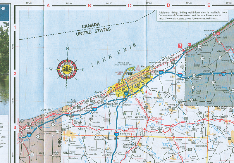
Far from being a "system," because it is unique every time it is used, an effective solution is create an arbitrary grid onto maps, like the "A, B, C,..." and "1, 2, 3,..." grid that is used on Pennsylvania Department of Transportation highway maps (PennDoT), like the one shown here:

Where is this entire map area within the world?

The second question is asking how you report the location of the map you are studying. This is not likely to be an issue if the map shows a large, easily recognized area such as the United States, the world, or even your home state. However, if the area is unfamiliar and smaller, such as one USGS quadrangle, then that becomes a challenge. As with the first question, there are several solutions to this task.

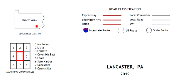
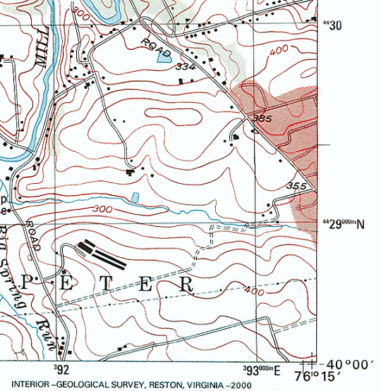
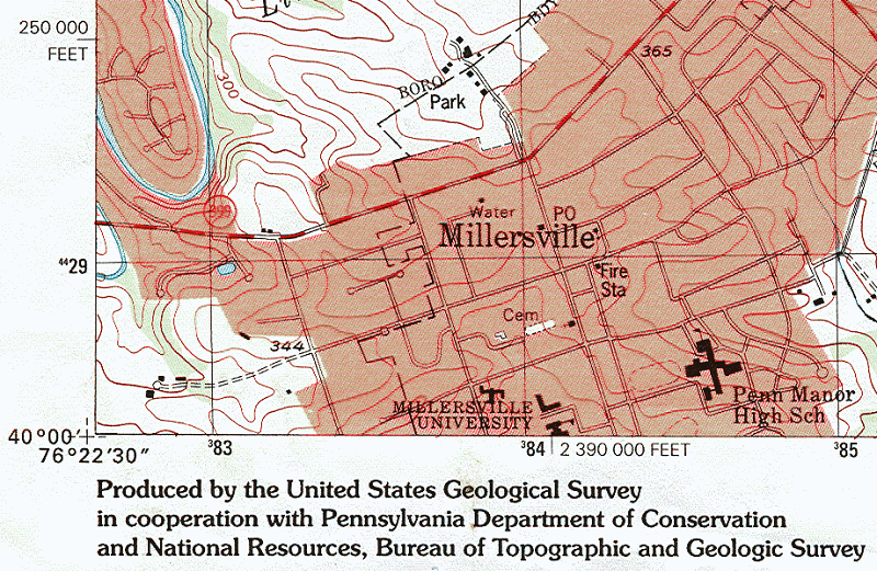
As with the previous question, there is a non-systematic solution to this question, too. Once again, it is unique every time it is used. The concept is to add an extra map to a corner of a larger map, in which the larger map is shown in a very small representation, and is shown surrounded by a larger recognizable area. The map shown below is the lower-right-hand corner of the Lancaster USGS topographic map (USGS), and uses two ways to let map readers know where the quadrangle area is relative to Pennsylvania and to the adjacent quadrangles.

Answers to the Questions

The options for answering the location questions include the following:

Keep in mind that the primary consideration for what will work for a given map depends on the map's purpose and audience. The scale of the map (derived from those considerations) determines whether some kinds of objects are points or areas; the best example of this phenomenon is the representation of towns on smaller scale maps as points versus their representation on larger scale maps as areas with definite boundaries.

• The Latitude-Longitude system, a non-Euclidean coordinate system
• Locator maps or map insets
• Arbitrary grid systems added to printed maps
• The UTM grid system, a plane geometry grid system
• The State Plane Coordinate System, another plane geometry grid system
• The Metes and Bounds Survey System, a system for identifying property parcels
• The US Public Land Survey System, another system for identifying property parcels
• The governing jurisdiction hierarchy of country, state, county (or parish), and any other minor civil divisions (townships, towns, boroughs, cities, etc.), based on named areas
• Postal addressing system
• The US National Grid and its predecessors

These options can be organized into three broad categories, which will be introduced in this unit and the next.

• Coordinate systems ("grids"): x-y coordinate systems to locate points
• Survey systems: land partitioning (subdivision) systems
• Naming or Designating systems: assigning names or categories

Accuracy vs. Precision

Highly relevant to discussions of maps is this pair of concepts you have probably been taught before, most likely in a science class. The difference in the context of maps is that they apply to locations (discussed here) and the distances between them (later). In general, location accuracy is the issue of how correctly a point is located: is it in the right location? Location precision is the issue of how detailed the point's location is: to how many decimal places are the numbers calculated?

Accuracy

The Case of Pillow. . . , or should that be The Pillow Case?

We tend to assume that the maps we use are accurate. But, inaccuracy can creep into a map from many sources. Surveying instruments might be miscalibrated, GPS satellite signals may experience atmospheric interference, or an assistant may write or type a wrong number.

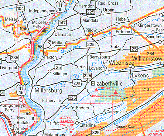
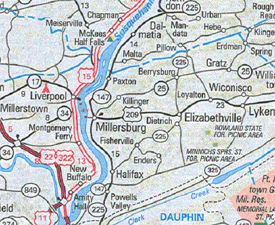
Compare these two map selections (I am intentionally keeping them anonymous). Find Pillow, PA on each map. In which county is Pillow located, to the north of the Dauphin County/Northumberland County boundary line, or to its south? The maps are showing that Pillow's location might be accurate on both maps, but the boundary is displayed differently.

Precision

Precision in maps is mostly dependent on the map's scale. A city whose location is recorded to the nearest whole degree might appear correct on a map of the whole country, but on a map of its county, one degree of latitude or longitude could easily represent the entire extent of the map. To represent the city's location realistically would require a location measured to the nearest minute (of latitude and longitude) or less. Without that additional precision, a latitude of 77° West longitude, 41° North latitude, the approximate location of Pillow, PA, would be read on a more detailed map as 77° 0' 0" W, 41° 0' 0" N, instead of its true location of 76° 48' 8" W, 40° 38' 24" N (USGS GNIS). Make sure you understand that, even though the result is an inaccurate location on the county map, the inaccuracy is entirely due to imprecision, not to any other cause.

Similarly, in our Pillow Case above, it is clear that the second map is less accurate at the scale at which both maps are being displayed here. The labels on the second map are displayed in a slightly larger font, which tells me that the second map is being displayed at a larger scale than was originally intended. So, at the smaller scale intended by the cartographer, the degree to which that small section of the county border was simplified was probably consistent with other accommodations for maps at that scale. Smaller scale maps are commonly less precise than larger scale maps.

Another Example

The example I have seen (and heard about from students) the most in other descriptions of the difference between Accuracy and Precision is one in which an archer shoots arrows at a target, as if the archer's skill is somehow tied to accuracy and precision. The archery example gives a completely wrong conception of these concepts and has the potential to mislead students into thinking that accuracy and precision are determined by their skill level in their scientific work.

Think instead of a weighing scale; I am thinking of a bathroom scale for weighing people, but the example is easily transferred to other size scales. Scale A gives the user their weight to the nearest half of a pound (to the nearest 0.5 pound). Scale B gives the user their weight to the fifth of a pound (to the nearest 0.2 pound). Scale B is therefore more precise than Scale A. There is nothing anyone can do to make Scale A more precise than it is (short of redesigning and rebuilding it). That does not mean, however, that Scale B is more accurate than Scale A. Scale B could be consistently over-reporting your weight by 0.6 pounds every time you use it, while Scale A is not. Of course, the only way to know that is if you weigh on both scales an object whose weight is known accurately and precisely.

Point-Based Coordinate Systems

Latitude and Longitude

The graticule, as it is referred to technically, is the most universal of the coordinate system options listed above. It is a global system, and yet a location reported to the nearest second of latitude and longitude is within 100 feet of its true location. Latitude and longitude locations are often reported to the nearest tenth or hundredth of a second, which makes them very precise indeed.

How Precise are Latitude-Longitude Coordinates?

The circumference of the Earth at the equator is roughly equal to the circumference of the Earth around any meridian-based great circle. Therefore, one degree of longitude along the equator is about the same as one degree of latitude along any meridian. That means that we can determine the minimum (worst) precision of the graticule by using calculations based on the equatorial circumference. The precision is better along any other parallel, because the length of that parallel will be shorter than the equator. The chart below simplifies the calculations by making them approximate in order to give answers with round numbers that are easier to remember.

Lat-Long Distance (of latitude at the equator)	Calculation	Precision
1 degree	25,000 miles/360 degrees	1 degree = approx. 70 miles
1 minute (1/60th of a degree)	70 miles/60 minutes	1 minute = approx. 1.1 mile 1 minute = approx. 6000 feet
1 second (1/60th of a minute)	6000 feet/60 seconds	1 second = approx. 100 feet
.1 second	100 feet/10 tenths	.1 second = approx. 10 feet

These calculations demonstrate that by giving a latitude-longitude location of an object to the nearest tenth of a second you are, at worst (on the equator) within 10 feet of that object.

Another Precise System: Decimal Degrees

You will hear several times how hard some organizations worked to come up with an alternative to the Latitude-Longitude system because of the awkwardness of working with degrees, minutes and seconds. The realm of GIS is one of those organizations because, as a computer technology, it was much easier to write programs for decimal-based number systems. One outcome was the development of the concept of decimal degrees. Decimal degrees keep the number of degrees in a latitude and longitude coordinate pair, but convert the rest of each coordinate (the minutes and seconds parts) into a decimal fraction of the whole degree.

For example:

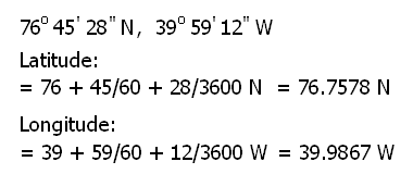
Since it is a minor problem for computers to have to deal with the North and South portion of a latitude, and the East and West portion of a longitude, the GIS software simplifies that part to positive and negative values. So, as stored in a computer, the above location would be: 76.7578°, -39.9867°.

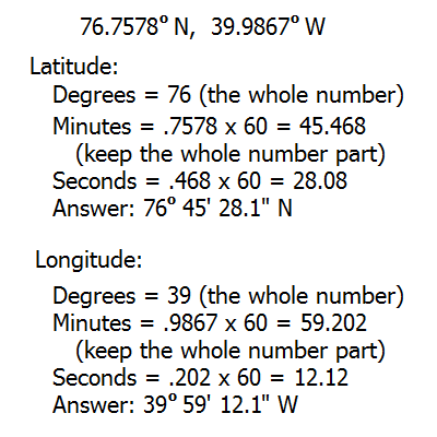
To reverse the procedure, and find the degrees, minutes and seconds expression of the location when you are given the decimal degrees, follow the steps illustrated below.

In terms of Accuracy and Precision, it is easy enough to demonstrate the decimal degree equivalents to the degrees-minutes-seconds values in the table above. One second of latitude is equivalent to 0.00028 decimal degrees and therefore a tenth of a second of latitude, which was comparable to 10 feet or less on the ground, corresponds to 0.000028 decimal degrees. Thus, a system of coordinates stored in decimal degrees to the sixth decimal place is capable of recording positions within a foot of their location on Earth.

The Universal Transverse Mercator Coordinate System

As a spherical coordinate system, we have seen, the latitude and longitude system is very efficient; however, it is awkward dealing with degrees, minutes and seconds, and even with the decimal equivalent (decimal degrees), as the units of measure. As a result, several alternative systems have been developed which take advantage of the simpler concepts of plane geometry.

The UTM grid is one such system, originating around the time of World War II with the US Army's main mapping unit, the Corps of Engineers. The UTM (Universal Transverse Mercator) coordinate system is a "plane" coordinate system, which means that it is designed to have true X and Y coordinates on a plane geometry grid. The only way to accomplish that is to first draw the map "projected," and then superimpose the plane geometry grid on that projected map. The purpose of a "map projection" is to reduce map distortion caused by the curvature of the Earth; you will learn about map projections in a forthcoming unit. The UTM coordinate system will be reexamined at that point. One advantage of the UTM coordinate system that you will see is its global coverage. One disadvantage to many Americans is that the global scope of the projection has led to its preference for metric units.

Map projections do not remove distortion due to the Earth's curvature completely. The best way to improve the projection's performance in this regard is to reduce the amount of the Earth covered by the projection. In this case, the adjustment made to accommodate that distortion was that created projected maps that were narrow but long strips only 6° of longitude wide. Then they repeated that narrow strip of projected map 60 times around the globe.

Each of the narrow projected maps is referred to as a UTM "zone." So, the format of the UTM Coordinate System is that it features separate coordinate systems customized for UTM zone; each separate coordinate system has its own (X = 0, Y = 0) starting point. The map below shows the UTM zones (with their number IDs) that occur in the continental US. The sixty zones start from 1 on the east side of the International Date Line and are counted (up to 60) as you move eastward around the globe.

Reading UTM Coordinates on USGS Quadrangles

Each UTM zone on the globe is divided into a North half and a South half, each of which in turn has its own coordinates. In addition, there is another set of coordinates based on a completely different approach for each polar region. Each of the long narrow half-zones has a set of coordinates that is measured from an origin that begins south and west of the zone, so that all measurements are positive when measuring to the east (referred to as Eastings) and positive when measuring to the north (called Northings). What adds to the uniqueness of the UTM system is the way the coordinates are displayed on the margins of the map (see the example below). Keep in mind that the width (east to west) of each zone is much less than its length south to north. The unique pattern of smaller and larger digits emphasizes the most significant digits. As the coordinates continue along the sides of the map every 1000 meters, the last three digits are simply dropped so that the labels are simply counting the thousands.

On the newer digital USGS quadrangles the 1,000 meter UTM grid is displayed using subtle yellow-orange lines. In the layer list available when viewing the quadrangles in Adobe Reader, they are the first legend item listed in the Map Frame set of layers. Reflecting the federal government's interest in all Americans becoming more aware of this system and one of its progeny, the US National Grid (see next unit), as well as more Americans learning the metric system of measurements, it is simply labeled "Projection and Grids" with no further identification.

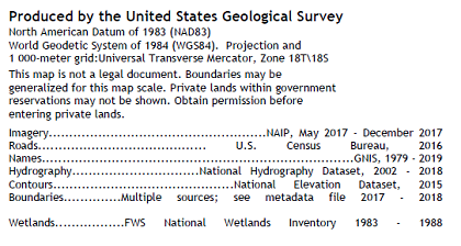
Here is the information presented about the UTM coordinate system in the lower left corner of a USGS quadrangle on two different versions of the same Lancaster, PA quadrangle. The first is one of the older scanned paper quadrangles, while the second is a newer digital version. In both cases the text includes a single line of text specifying that the 1000-meter UTM grid is present and that Lancaster is in zone 18. The "18T/18S" on the 2019 Lancaster quadrangle is a nod to the US National Grid, which will be introduced in the next unit.

That is all we are going to learn about the UTM coordinate system in this course. There is a great deal more detail to it, but because it is not used much in the civilian world, there is a strong chance that you will not encounter it. You should be able to recognize its connection to Grid North in the declination diagram (more about that will come later), and be able to explain the meaning of its unusually-presented coordinates around the margins of the USGS quadrangles.

The US State Plane Coordinate System

The State Plane Coordinate System is also a plane coordinate system, similar to the UTM system in that it is designed to express coordinates as X,Y values on a plane geometry grid. The purpose of the State Plane Coordinate System is to create separate coordinate systems customized for each US state.

Since those coordinate systems are to be laid out on a flat plane, there must first be a way to adapt the round Earth to that flat surface. That is the concept behind what are known as "map projections." We will investigate map projections much more deeply very soon in this course, but for now assume that there is a map projection, and therefore a coordinate system, optimized for each US state. Generally, there are many possible types of map projections, though only a relatively small number of those types are suited to our region of the world. No map projection produces a completely undistorted map, but projections of such smaller areas will be much less distorted than projections of larger areas; thus, we can reduce distortion better for a state than we can for the entire US.

As we saw with the UTM coordinate system, each State Plane Coordinate System zone is measured from its own origin (X = 0, Y = 0) that begins south and west of the zone, so that all coordinates are positive Eastings and positive Northings. The ground distance units for the map scales are usually feet, although there are some cases in which metric units are now being applied.

To make things a little more complicated, in the larger states one map projection cannot cover the entire state without too much local distortion of distance, angle or area in some parts of the state. For those states, the state was divided into "zones," each of which has its own State Plane Coordinate system; Pennsylvania has two such zones, for example. So, it is tricky enough that you have to start a new coordinate system, with its own (X = 0, Y = 0) starting point, when you cross from one state to the next, but you also have to do that within states, too, when you cross from one zone to the next.

The State Plane Coordinate System (SPCS) saw a great deal of use with the introduction of GIS (Geographic Information Systems) software, primarily with local governments who adopted the technology. In fact Lancaster County, PA was an early adopter of GIS who has built a very expensive and powerful GIS system. In order to specify locations for all of the objects in the county that they have mapped, including such items as houses, fire hydrants and property lines, they use state plane coordinates measured in feet. The biggest advantage to using it was the precision that could be maintained with feature locations recorded to the nearest foot.

The SPCS on USGS Quadrangles

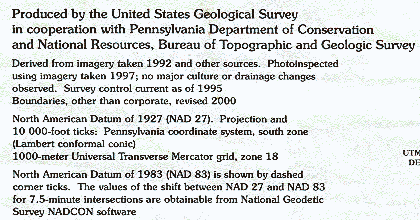
The coordinates of the SPCS were displayed very simply on older USGS quadrangles (see the example below) compared to how the UTM grid is displayed. In fact, only the southwest and northeast corners of the USGS maps generally contained SPCS reference labels. This "grid" is described in the marginal text in the lower left corner of any USGS topographic quadrangle. Below is that text from one of the older editions of the Lancaster, PA quadrangle. Look for the references to the "Pennsylvania coordinate system, south zone" and the "10 000-foot ticks."

The State Plane grid is also not visible within the map, but there are several markings (the "grid ticks" that the text shown above referred to) around the edge of the map. The markings are placed 10,000 feet apart around the map edge, but only two of them are labeled (see below). The rationale from the perspective of the USGS is that the quadrangle contains a map scale in feet, so users can find any location with those pieces of information.

Interestingly, the same presentation of those coordinates and statement of their context was included on the 2013 and 2016 digital versions of the Lancaster quadrangle, but the State Plane Coordinate System is completely absent from the 2019 version. The decision was made in 2017, but the USGS website does not include an explanation of why.

The National Geodetic Survey website does provide a clue, however. It appears that State Plane Coordinates are a system in transition. Since 2018, steps have been taken to update the North American Datum definition last updated around 1983. A major revision is due to become official in 2022. Since State Plane Coordinates are referenced relative to fixed latitude-longitude locations, they too will have to be adjusted. In fact, Pennsylvania and other states are considering eliminating their existing State Plane Coordinate System zones in favor of maps of smaller zones with more detailed data recorded in more heavily populated and developed areas. This is still very much a "work in progress."

The concept of "datum" will be addressed later in this course, but the above view of the southwest corner of the Lancaster quadrangle from 1997 illustrates the difference. At that stage in the production of the paper quadrangles, updates were simply added to previously drawn quadrangles. The updated 1983 datum was a modification to the previous 1927 datum in much the same way that the 2022 modifications will be. That corner of the quadrangle includes a crosshairs symbol at the southwest corner of the quadrangle that indicates how much everything on the quadrangle should have shifted if the quadrangle had been completely redrawn from scratch. Most likely, with an all-digital processing system, such adjustments will not be necessary for the newer 2022 datum changes.

Locations on USGS Quadrangles

Locations on Paper Quadrangles

The primary value of USGS quadrangles has always been based on their precision and accuracy for relatively large-scale mapping. With data originating from "rectified" aerial photographs and the readily available third dimension of elevation (we will investigate contour lines thoroughly later in this course), the USGS quadrangles are widely respected for their quality. Of course, in earlier times, taking advantage of those qualities meant learning manual techniques for calculating precise latitudes and longitudes from the paper quadrangles, or using the available grids for UTM coordinates or State Plane coordinates.

Those measurement skills for calculating latitude-longitude locations depended on either measuring or estimating the horizontal position of a desired point between two known latitudes or the vertical position of a desired point between two known longitudes on the paper quadrangle. That paper distance measured in inches could then be reduced to a proportion of the difference in the two known latitudes (or longitudes). You will see just below that you no longer need to make such precise measurements and calculations, but it is still useful sometimes to be able to estimate such locations.

Locations on Digital Quadrangles

Now that the quadrangles are digital, we have digital tools for achieving those same precise latitudes and longitudes.

When the PDF version of the quadrangles was introduced earlier in this course, we found the "Measure" tools in the Adobe Reader app: with one GeoPDF file open in Adobe Reader three tabs appear above the map and below the program menus. The second of those tabs is the “Tools” tab. Click on it and choose to open the "Measure" tools. The names of three tools become visible just above the map: Measuring Tool, Object Data Tool, and Geospatial Location Tool. For the topic we are currently considering, the Geospatial Location Tool is the most appropriate.

Click on the name of the Geospatial Location Tool and a small gray box will appear in the lower right corner of the map viewing area. Initially it only says "Latitude:" and "Longitude:" but as you move your mouse cursor back over the map you will see numbers appear after the labels. The numbers are decimal degree values for latitude and longitude (respectively) for almost any location within the map area. The only place where the tool is a little unreliable is along the edges and at the very corners of the rectangle surrounding the map. The values presented in the gray box are numerical to four decimal places. They give latitudes as positive numbers in the US with no indication that these are North latitudes, and they give longitudes as negative numbers in the US with no indication that these are West longitudes.

How precise is a latitude or longitude degree measurement to four decimal places? A change in latitude of 0.0001 degree is equivalent to about 0.4 seconds of latitude. As noted above, that is equivalent to about 40 feet. The comparable change for a longitude measurement will be less, except at the equator where it will be the same as it is for latitude. The longitude change for a difference of 0.0001 degree will decrease gradually from the equator toward either pole, reaching zero at the pole.

GIS Coordinate Systems

Coordinate Systems in GIS Software

GIS specialists benefit from understanding such concepts as coordinate systems, map projections, scale, and other map basics. Maps are stored in a computer as a collection of points. The points are identified in the spatial data file as either isolated points, points along a line, or points along an area's boundary. Each point is stored as a pair of coordinates.

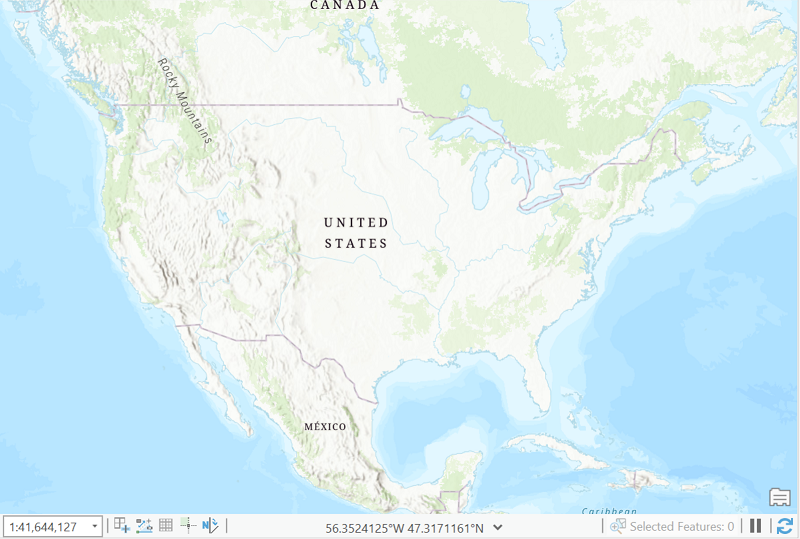
The coordinate system underlying a map is undefined when GIS software is first opened. The lower right corner of the image below states the coordinates in the blank view are "unknown."

Later in this course you will learn that several different coordinate systems appear on topographic maps: latitude-longitude coordinates (in degrees, minutes and seconds), State Plane coordinates (in feet) and UTM coordinates (in meters). We will also see that latitude-longitude degrees-minutes-seconds coordinates can be converted to decimal degrees, which is far better suited to the computer environment, but is a challenge for those who were brought up on degrees, minutes and seconds.

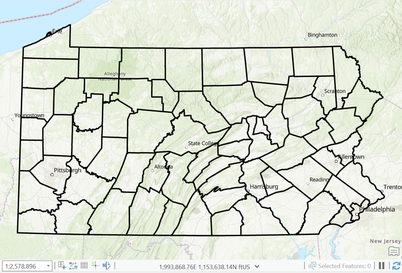
In this next image, one layer of Pennsylvania counties has been added to the map. Notice that in the lower right corner of the ArcGIS window the software displays the current position of the cursor in decimal degrees.

Coordinate System Choices

Is one coordinate system better than the others? It depends on the context. For representing world maps on the computer, latitude-longitude is the only one that makes sense. The UTM coordinate system works for a large area, including some countries, that is within one UTM zone. The computer can handle the calculations involved in representing an area that is in the overlap between two UTM zones, but it is not necessarily easy for the user to make quick sense of it or to use those coordinates for calculations. UTM coordinate systems make sense also for users in countries that depend on metric measurements.

State Plane coordinates are relevant only for American map areas; Canada has a similar set of provincial coordinate systems, but this is not a standard among countries. The fact that our State Plane coordinates are measured in feet increases their appeal to American GIS users. Once again, though, they make little sense for areas that extend across state boundaries, since you are then in an overlap between two sets of coordinates in the same units. The State Plane coordinate system in the bigger states is divided into several zones; for example, Pennsylvania has a North Zone and a South Zone. That means that it is impractical for Pennsylvania to use the State Plane coordinate system for statewide mapping. State Plane coordinates make the most sense for smaller areas such as counties.

The only shortcoming is if any GIS organization tied to a particular set of boundaries needs to share data with surrounding areas outside of their own boundaries. In that context, the best fallback is the decimal degrees for the latitude-longitude coordinates system.

Spatial Data Tables

Adding Table Data

We have made the points that all GIS data must be stored in data files using a standard, specified coordinate system, and that GIS data are added to ArcGIS Pro as shapefiles. The purpose of this next discussion is to demonstrate that neither of those points is necessarily true. There are, in fact, multiple file formats that ArcGIS can read and import data from, and it is possible to add data that are attribute-based, not just location-based. Note: you are not going to be shown all the options, just some that will have practical applications for users from a wide range of disciplines.

Excel File Characteristics

The examples start with adding data stored in an Excel spreadsheet file or another more generic text file to the map, though other formats can be used to store similar data. In order to understand the import process on the ArcGIS side of this procedure, there are a few characteristics and capabilities of Excel that will be important to know.

The first is that Excel can store both text data and numerical data. Furthermore, Excel always attempts to identify what type of data is present in any spreadsheet cell. When Excel identifies a cell's contents as text, it will left-justify those contents; when it contains what are obviously numerical values, it right justifies them. Anything that is not an obvious number will be treated as text.

Next, recognize some Excel terminology. Excel displays one "worksheet" at a time but can include many worksheets. The worksheets are switched by clicking on their tabs at the bottom of the Excel window. The collection of worksheets that makes up an Excel file is referred to as a "workbook."

Text File Characteristics

Excel has its own custom file format, in which files are saved with a filename extension "XLSX," similar to how a Microsoft Word file has a DOCX filename extension. Excel can also open files which are generic text files, particularly those whose filename extension is CSV. Scanners that can read a document and convert the image into text content (which can include letters and numbers) might save the results in a text file format by default; just remember that CSV is the preferred type. If the scanner is able to convert the scanned content to a Word file format, Word can save its files as text files. What is special about a CSV file is that, as it stores the content of one row of data, it inserts a comma between the contents of consecutive cells in that row (CSV is short for Comma-Separated Values). Excel readily opens that format which can make it easier to then manipulate the data in many ways. Excel can then save files in either XLSX or CSV format.

In addition to scanners, other technologies save data in the CSV format. GPS devices, environmental data gathering equipment at fixed locations and survey results from online questionnaires are likely candidates, and there are others. Store the CSV or XLSX data file in the same folder with your shapefiles or other GIS data.

ArcGIS's Requirements

The file contents must conform to what ArcGIS can work with. Like the geographer's data table and the ArcGIS Pro attribute table that we have already covered, the rows must represent map features and the columns must represent data variables or fields. Furthermore, the first row must contain the variable names and the data within each column must start in row 2.

ArcGIS can accept either CSV or XLSX files as inputs. Use the same Add Data dialog that opens shapefiles. When a CSV file is detected it is imported as a "table." When an XLSX file is detected there is one more step; ArcGIS cannot open an Excel workbook, but it can open a worksheet; so, double-click on the workbook and select the worksheet (even if it is the only worksheet in the workbook). Again, the worksheet is imported as a table.

Add and Display X-Y Data

Create the Points Layer

If you have data columns containing latitude-longitude coordinates, such as data produced by a GPS device, make sure the latitude column name is LATITUDE or Y, and the longitude data column is LONGITUDE or X (it does not have to be in all capital letters). Otherwise, there will be later steps where you need to identify which column is each of those. When adding the table, one option is Add XY Data. Choose it and ArcGIS Pro will recognize it as a potential spatial layer. If you have not used the default spatial column names, this will be an opportunity to identify them. You will also specify which coordinate system the data are stored in.

The expectation is that the data are going to be displayed as point locations on your map. If that is not the intended use, there are tools within ArcGIS for creating lines or areas from the points, but that is beyond our scope here.

If you do not add the data table as an XY Data table, you can still add it as an ordinary collection of variables corresponding to a collection of map features (more on that below). In that case, you will still be able to display the point features.

Once the table appears in the Contents list in ArcGIS Pro right click on it. Because it is a table and not a shapefile-based layer, the menu that drops down is different. One of the choices is "Display XY Data..." that will create a new points layer and add it to the Table of Contents.

Other Data Table Uses

Another use of tabular data is simply to add fields to an existing layer, whether points, lines or areas. The data table has to meet certain requirements, but it can then be "joined" or "related" to the existing layer. We are not digging that deeply into ArcGIS Pro here, but you can either look up the instructions or take the Geography Department's GIS course to learn more.

The final way to use a data table to create a GIS layer is called "Geocoding" (again, beyond our scope here). There are several forms of geocoding, depending on the types of data and your purpose. For example, one form of geocoding starts with a group of columns that combine to form home or business addresses, including variables such as house number, street name and zip code. It requires a layer of roads broken into short road segments equivalent to city blocks that have data such as the highest and lowest address number on both sides of the street, the name and type of street (road, avenue, lane, etc.), and the zip code. ArcGIS will estimate the location of each house on the correct side of the road.

There are quite a few other geocoding strategies built into the software as well.