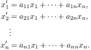
Here is a system of n differential equations in n unknowns:
This is a constant coefficient linear homogeneous
system. Thus, the coefficients ![]() are constant, and
you can see that the equations are linear in the variables
are constant, and
you can see that the equations are linear in the variables ![]() ,
...,
,
..., ![]() and their derivatives. The reason for the term
"homogeneous" will be clear when I've written the system in
matrix form.
and their derivatives. The reason for the term
"homogeneous" will be clear when I've written the system in
matrix form.
The primes on ![]() , ...,
, ..., ![]() denote differentiation with respect to an
independent variable t. The problem is to solve for
denote differentiation with respect to an
independent variable t. The problem is to solve for ![]() ,
...,
,
..., ![]() in terms of t.
in terms of t.
Write the system in matrix form as
![$$\left[\matrix{x_1' \cr \vdots \cr x_n' \cr}\right] = \left[\matrix{a_{11} & \cdots & a_{1n} \cr a_{21} & \cdots & a_{2n} \cr \vdots & & \vdots \cr a_{n1} & \cdots & a_{nn} \cr}\right] \left[\matrix{x_1 \cr \vdots \cr x_n \cr}\right].$$](system9.png)
Equivalently,
![]()
(A nonhomogeneous system would look like ![]() .)
.)
It's possible to solve such a system if you know the eigenvalues (and possibly the eigenvectors) for the coefficient matrix
![$$\left[\matrix{a_{11} & \cdots & a_{1n} \cr a_{21} & \cdots & a_{2n} \cr \vdots & & \vdots \cr a_{n1} & \cdots & a_{nn} \cr}\right]$$](system12.png)
First, I'll do an example which shows that you can solve small linear systems by brute force.
Example. Consider the system of differential equations
![]()
![]()
The idea is to solve for ![]() and
and ![]() in terms of t.
in terms of t.
One approach is to use brute force. Solve the first equation for ![]() ,
then differentiate to find
,
then differentiate to find ![]() :
:
![]()
Plug these into second equation:
![]()
This is a constant coefficient linear homogeneous equation in ![]() .
The characteristic equation is
.
The characteristic equation is ![]() . The roots are
. The roots are ![]() and
and ![]() . Therefore,
. Therefore,
![]()
Plug back in to find ![]() :
:
![]()
The procedure works, but it's clear that the computations would be pretty horrible for larger systems.
To describe a better approach, look at the coefficient matrix:
![]()
Find the eigenvalues:
![]()
This is the same polynomial that appeared in the example. Since ![]() , the
eigenvalues are
, the
eigenvalues are ![]() and
and ![]() .
.
Thus, you don't need to go through the process of eliminating ![]() and
isolating
and
isolating ![]() . You know that
. You know that
![]()
once you know the eigenvalues of the coefficient matrix. You
can now finish the problem as above by plugging ![]() back in to solve for
back in to solve for ![]() .
.
This is better than brute force, but it's still cumbersome if the system has more than two variables.
I can improve things further by making use of eigenvectors as well as eigenvalues. Consider the system
![]()
Suppose ![]() is an eigenvalue of A with eigenvector v. This means
that
is an eigenvalue of A with eigenvector v. This means
that
![]()
I claim that ![]() is a solution to the equation,
where c is a constant. To see this, plug it in:
is a solution to the equation,
where c is a constant. To see this, plug it in:
![]()
To obtain the general solution to ![]() , you
should have "one arbitrary constant for each
differentiation". In this case, you'd expect n arbitrary
constants. This discussion should make the following result
plausible.
, you
should have "one arbitrary constant for each
differentiation". In this case, you'd expect n arbitrary
constants. This discussion should make the following result
plausible.
![]()
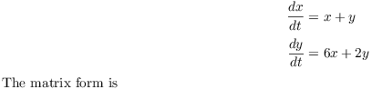
Example. Solve
![]()
![]()
The matrix form is
![]()
The matrix
![]()
has eigenvalues ![]() and
and ![]() . I need to find the
eigenvectors.
. I need to find the
eigenvectors.
Consider ![]() :
:
![]()
The last matrix says ![]() , or
, or ![]() . Therefore,
. Therefore,
![]()
Take ![]() . The eigenvector is
. The eigenvector is ![]() .
.
Now consider ![]() :
:
![$$A - 3I = \left[\matrix{-32 & -48 \cr 16 & 24 \cr}\right] \quad \rightarrow \quad \left[\matrix{1 & \dfrac{3}{2} \cr \noalign{\vskip2pt} 0 & 0 \cr}\right]$$](system64.png)
The last matrix says ![]() , or
, or ![]() .
Therefore,
.
Therefore,
![$$\left[\matrix{a \cr b \cr}\right] = \left[\matrix{-\dfrac{3}{2}b \cr \noalign{\vskip2pt} b \cr}\right] = b \left[\matrix{-\dfrac{3}{2} \cr \noalign{\vskip2pt}1 \cr}\right].$$](system67.png)
Take ![]() . The eigenvector is
. The eigenvector is ![]() .
.
You can check that the vectors ![]() ,
, ![]() , are independent.
Hence, the solution is
, are independent.
Hence, the solution is
![]()
Example. Find the general solution ![]() to the linear system
to the linear system
![]()
Let
![]()
![]()
The eigenvalues are ![]() and
and ![]() .
.
For ![]() , I have
, I have
![]()
If ![]() is an eigenvector, then
is an eigenvector, then
![]()
So
![]()
![]() is an eigenvector.
is an eigenvector.
For ![]() , I have
, I have
![]()
If ![]() is an eigenvector, then
is an eigenvector, then
![]()
So
![]()
![]() is an eigenvector.
is an eigenvector.
The solution is
![]()
Example. ( Complex roots) Solve
![]()
![]()
The characteristic polynomial is
![]()
The eigenvalues are ![]() . You can check that the
eigenvectors are:
. You can check that the
eigenvectors are:
![$$ \eqalign { \lambda = 1 - 2i: \quad & b\cdot \left[\matrix{-2 + i \cr 2 \cr}\right]\cr \lambda = 1 + 2i: \quad & b\cdot \left[\matrix{-2 - i \cr 2 \cr}\right]\cr } $$](system97.png)
Observe that the eigenvectors are conjugates of one another. This is always true when you have a complex eigenvalue.
The eigenvector method gives the following complex solution:
![]()
![]()
Note that the constants occur in the combinations ![]() and
and ![]() . Something like this will
always happen in the complex case. Set
. Something like this will
always happen in the complex case. Set ![]() and
and ![]() . The solution is
. The solution is
![]()
In fact, if you're given initial conditions for ![]() and
and ![]() , the new constants
, the new constants ![]() and
and ![]() will turn out to be real numbers.
will turn out to be real numbers.![]()
You can get a picture of the solution curves for a system ![]() even if you can't solve it by sketching the direction field. Suppose you have a two-variable
linear system
even if you can't solve it by sketching the direction field. Suppose you have a two-variable
linear system
![]()
This is equivalent to the equations
![]()
Then
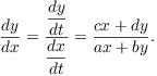
That is, the expression on the right gives the
slope of the solution curve at the point ![]() .
.
To sketch the direction field, pick a set of sample points --- for
example, the points on a grid. At each point ![]() , draw the vector
, draw the vector
![]() starting at the point
starting at the point ![]() . The collection of vectors is the direction field. You can
approximate the solution curves by sketching in curves which are
tangent to the direction field.
. The collection of vectors is the direction field. You can
approximate the solution curves by sketching in curves which are
tangent to the direction field.
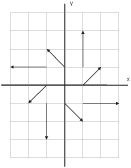
Example. Sketch the direction field for
![]()
I've computed the vectors for 9 points:
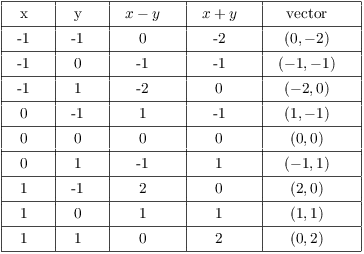
Thus, from the second line of the table, I'd draw the vector ![]() starting at the point
starting at the point ![]() .
.
Here's a sketch of the vectors:
While it's possible to plot fields this way, it's very tedious. You can use software to plot fields quickly. Here is the same field as plotted by Mathematica:
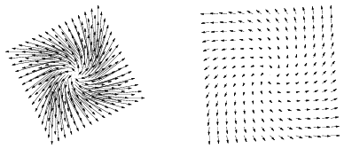
The first picture shows the field as it would be if you plotted it by hand. As you can see, the vectors overlap each other, making the picture a bit ugly. The second picture is the way Mathematica draws the field by default: The vectors' lengths are scaled so that the vectors don't overlap. In subsequent examples, I'll adopt the second alternative when I display a direction field picture.
The arrows in the pictures show the direction of increasing t on the
solution curves. You can see from these pictures that the solution
curves for this system appear to spiral out from the origin.![]()
Example. ( A compartment model) Two tanks hold 50 gallons of liquid each. The first tank starts with 25 pounds of dissolved salt, while the second starts with pure water. Pure water flows into the first tank at 3 gallons per minute; the well-stirred micture flows into tank 2 at 4 gallons per minute. The mixture in tank 2 is pumped back into tank 1 at 1 gallon per minute, and also drains out at 3 gallons per minute. Find the amount of salt in each tank after t minutes.
Let x be the number of pounds of salt dissolved in the first tank at time t and let y be the number of pounds of salt dissolved in the second tank at time t. The rate equations are
![]()
![]()
Simplify:
![]()
Next, find the characteristic polynomial:
![]()
The eigenvalues are ![]() ,
, ![]() .
.
Consider ![]() :
:
![$$A + 0.04I = \left[\matrix{-0.04 & 0.02 \cr 0.08 & -0.04 \cr}\right] \quad \rightarrow \quad \left[\matrix{1 & -\dfrac{1}{2} \cr \noalign{\vskip2pt} 0 & 0 \cr}\right]$$](system130.png)
This says ![]() , so
, so ![]() .
Therefore,
.
Therefore,
![$$\left[\matrix{a \cr b \cr}\right] = \left[\matrix{\dfrac{1}{2}b \cr \noalign{\vskip2pt} b \cr}\right] = b\left[\matrix{\dfrac{1}{2} \cr \noalign{\vskip2pt} 1 \cr}\right].$$](system133.png)
Set ![]() . The eigenvector is
. The eigenvector is ![]() .
.
Now consider ![]() :
:
![$$A + 0.12I = \left[\matrix{0.04 & 0.02 \cr 0.08 & 0.04 \cr}\right] \quad \rightarrow \quad \left[\matrix{1 & \dfrac{1}{2} \cr \noalign{\vskip2pt} 0 & 0 \cr}\right]$$](system137.png)
This says ![]() , so
, so ![]() .
Therefore,
.
Therefore,
![$$\left[\matrix{a \cr b \cr}\right] = \left[\matrix{-\dfrac{1}{2}b \cr \noalign{\vskip2pt}b \cr}\right] = b\left[\matrix{-\dfrac{1}{2} \cr \noalign{\vskip2pt}1 \cr}\right].$$](system140.png)
Set ![]() . The eigenvector is
. The eigenvector is ![]() .
.
The solution is
![]()
When ![]() ,
, ![]() and
and ![]() . Plug in:
. Plug in:
![]()
Solving for the constants, I obtain ![]() ,
, ![]() . Thus,
. Thus,
![]()
The direction field for the system is shown in the first picture. In the second picture, I've sketched in some solution curves.
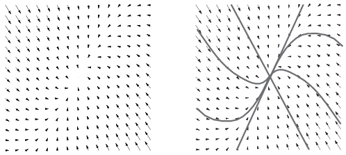
The solution curve picture is referred to as the phase portrait.
The eigenvectors ![]() and
and ![]() have slopes 2 and -2,
respectively. These appear as the two lines (linear solutions).
have slopes 2 and -2,
respectively. These appear as the two lines (linear solutions).![]()
Consider the linear system
![]()
Suppose it has has conjugate complex eigenvalues ![]() ,
, ![]() with eigenvectors
with eigenvectors ![]() ,
, ![]() , respectively. This yields solutions
, respectively. This yields solutions
![]()
If ![]() is a complex number,
is a complex number,
![]()
![]()
I'll apply this to ![]() , using the fact that
, using the fact that
![]()
Then
![]()
![]()
The point is that since the terms on the right are independent solutions, so are the terms on the left. The terms on the left, however, are real solutions. Here is what this means.
Example. Solve the system
![]()
![]()
Set
![]()
The eigenvalues are ![]() .
.
Consider ![]() :
:
![]()
The last matrix says ![]() , so
, so ![]() . The eigenvectors
are
. The eigenvectors
are
![]()
Take ![]() . This yields the eigenvector
. This yields the eigenvector ![]() .
.
Write down the complex solution
![]()
Take the real and imaginary parts:
![]()
![]()
The general solution is
![]()
The eigenvector method produces a solution to a (constant coefficient homogeneous) linear system whenever there are "enough eigenvectors". There might not be "enough eigenvectors" if the characteristic polynomial has repeated roots.
I'll consider the case of repeated roots with multiplicity two or three (i.e. double or triple roots). The general case can be handled by using the exponential of a matrix.
Consider the following linear system:
![]()
Suppose ![]() is an eigenvalue of A of multiplicity 2, and
is an eigenvalue of A of multiplicity 2, and ![]() is an eigenvector for
is an eigenvector for ![]() .
. ![]() is
one solution; I want to find a second independent solution.
is
one solution; I want to find a second independent solution.
Recall that the constant coefficient equation ![]() had independent solutions
had independent solutions ![]() and
and ![]() .
.
By analogy, it's reasonable to guess a solution of the form
![]()
Here ![]() is a constant vector.
is a constant vector.
Plug the guess into ![]() :
:
![]()
Compare terms in ![]() and
and ![]() on the left
and right:
on the left
and right:
![]()
While it's true that ![]() is a solution,
it's not a very useful solution. I'll try again, this time
using
is a solution,
it's not a very useful solution. I'll try again, this time
using
![]()
Then
![]()
Note that
![]()
Hence,
![]()
Equate coefficients in ![]() ,
, ![]() :
:
![]()
![]()
In other words, ![]() is an eigenvector, and
is an eigenvector, and ![]() is a vector which is mapped by
is a vector which is mapped by ![]() to the eigenvector.
to the eigenvector. ![]() is called a generalized eigenvector.
is called a generalized eigenvector.
Example. Solve
![]()
![]()
Therefore, ![]() is an eigenvalue of multiplicity 2.
is an eigenvalue of multiplicity 2.
Now
![]()
The last matrix says ![]() , or
, or ![]() . Therefore,
. Therefore,
![]()
Take ![]() . The eigenvector is
. The eigenvector is ![]() . This gives a
solution
. This gives a
solution
![]()
Next, I'll try to find a vector ![]() such that
such that
![]()
Write ![]() . The equation becomes
. The equation becomes
![]()
Row reduce:
![$$\left[\matrix{-4 & -8 & -2 \cr 2 & 4 & 1 \cr}\right] \quad \rightarrow \quad \left[\matrix{1 & 2 & \dfrac{1}{2} \cr \noalign{\vskip2pt} 0 & 0 & 0 \cr}\right]$$](system225.png)
The last matrix says that ![]() , so
, so ![]() . In this situation, I may take
. In this situation, I may take ![]() ; doing so produces
; doing so produces ![]() .
.
This work generates the solution
![$$t e^t \left[\matrix{-2 \cr 1 \cr}\right] + e^t \left[\matrix{\dfrac{1}{2} \cr \noalign{\vskip2pt} 0 \cr}\right].$$](system230.png)
The general solution is
![$$\vec x = c_1 e^t \left[\matrix{-2 \cr 1 \cr}\right] + c_2 \left(t e^t \left[\matrix{-2 \cr 1 \cr}\right] + e^t \left[\matrix{\dfrac{1}{2} \cr \noalign{\vskip2pt} 0 \cr}\right]\right).$$](system231.png)
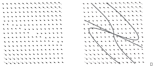
The first picture shows the direction field; the second shows the phase portrait, with some typical solution curves. This kind of phase portrait is called an improper node.
Example. Solve the system
![$$\vec x\,' = \left[\matrix{1 & 0 & 0 \cr 1 & 1 & 0 \cr 2 & -1 & 2 \cr}\right] \vec x.$$](system233.png)
The eigenvalues are ![]() and
and ![]() (double).
(double).
I'll do ![]() first.
first.
![$$A - 2I = \left[\matrix{-1 & 0 & 0 \cr 1 & -1 & 0 \cr 2 & -1 & 0 \cr}\right] \to \left[\matrix{1 & 0 & 0 \cr 0 & 1 & 0 \cr 0 & 0 & 0 \cr}\right]$$](system237.png)
The last matrix implies that ![]() and
and ![]() , so the
eigenvectors are
, so the
eigenvectors are
![$$\left[\matrix{a \cr b \cr c \cr}\right] = \left[\matrix{0 \cr 0 \cr c \cr}\right] = c\cdot \left[\matrix{0 \cr 0 \cr 1 \cr}\right].$$](system240.png)
For ![]() ,
,
![$$A - I = \left[\matrix{0 & 0 & 0 \cr 1 & 0 & 0 \cr 2 & -1 & 1 \cr}\right] \to \left[\matrix{1 & 0 & 0 \cr 0 & 1 & -1 \cr 0 & 0 & 0 \cr}\right]$$](system242.png)
The last matrix implies that ![]() and
and ![]() , so the
eigenvectors are
, so the
eigenvectors are
![$$\left[\matrix{a \cr b \cr c \cr}\right] = \left[\matrix{0 \cr c \cr c \cr}\right] = c\cdot \left[\matrix{0 \cr 1 \cr 1 \cr}\right].$$](system245.png)
I'll use ![]() .
.
Next, I find a generalized eigenvector ![]() . It
must satisfy
. It
must satisfy
![]()
That is,
![$$\left[\matrix{0 & 0 & 0 \cr 1 & 0 & 0 \cr 2 & -1 & 1 \cr}\right] \left[\matrix{a' \cr b' \cr c' \cr}\right] = \left[\matrix{0 \cr 1 \cr 1 \cr}\right].$$](system249.png)
Solving this system yields ![]() ,
, ![]() . I can take
. I can take
![]() , so
, so ![]() , and
, and
![$$\vec w = \left[\matrix{a' \cr b' \cr c' \cr}\right] = \left[\matrix{1 \cr 1 \cr 0 \cr}\right].$$](system254.png)
The solution is
![$$\vec x = c_1 e^{2t} \left[\matrix{0 \cr 0 \cr 1 \cr}\right] + c_2 e^t \left[\matrix{0 \cr 1 \cr 1 \cr}\right] + c_2 \left(te^t \left[\matrix{0 \cr 1 \cr 1 \cr}\right] + e^t \left[\matrix{1 \cr 1 \cr 0 \cr}\right]\right).\quad\halmos$$](system255.png)
I'll give a brief description of the situation for an eigenvalue ![]() of multiplicity 3. First, if there are three {\it
independent} eigenvectors
of multiplicity 3. First, if there are three {\it
independent} eigenvectors ![]() ,
, ![]() ,
, ![]() , the solution is
, the solution is
![]()
Suppose there is one independent eigenvector, say ![]() . One solution is
. One solution is
![]()
Find a generalized eigenvector ![]() by solving
by solving
![]()
A second solution is
![]()
Next, obtain another generalized eigenvector ![]() by solving
by solving
![]()
A third independent solution is
![]()
Finally, combine the solutions to obtain the general solution.
The only other possibility is that there are two independent
eigenvectors ![]() and
and ![]() . These give solutions
. These give solutions
![]()
Find a generalized eigenvector ![]() by solving
by solving
![]()
The constants a and b are chosen so that the equation is solvable.
![]() yields the solution
yields the solution
![]()
The best way of explaining why this works involves something called the Jordan canonical form for matrices. It's also possible to circumvent these technicalities by using the exponential of a matrix.
Send comments about this page to: Bruce.Ikenaga@millersville.edu.
Copyright 2015 by Bruce Ikenaga