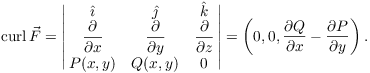
Theorem. If ![]() is a vector field in the plane,
and P and Q have continuous partial derivatives on a region. the
following four statements are equivalent:
is a vector field in the plane,
and P and Q have continuous partial derivatives on a region. the
following four statements are equivalent:
1. ![]() for some function
for some function ![]() .
.
2. ![]() .
.
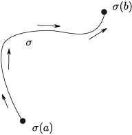
3. If ![]() is a closed curve
lying in the region --- i.e. a path which starts and ends at the same
point --- then
is a closed curve
lying in the region --- i.e. a path which starts and ends at the same
point --- then
![]()
4. ( Path independence) If ![]() and
and ![]() are paths in the region which start
at the same point and end at the same point, then
are paths in the region which start
at the same point and end at the same point, then
![]()
To say that these statements are equivalent means that if one of them is true, then all of them are true (and if one of them is false, all of them are false). A field that satisfies any one of these conditions is a conservative field --- or sometimes a gradient field, or sometimes path independent.
Before I show that these statements are equivalent, I'll give a couple of examples.
Example. Show that ![]() is a gradient field.
is a gradient field.
I want a function f such that ![]() , i.e.
, i.e.
![]()
Integrate the first equation with respect to x:
![]()
Since the integral is with respect to x, y is constant, and must be
included in the arbitrary constant --- hence ![]() . Differentiate with respect to y and set the result
equal to
. Differentiate with respect to y and set the result
equal to ![]() above:
above:
![]()
I get ![]() , so
, so ![]() . This time, D is a numerical
constant. Since the derivative of a number is 0, and since I just
want some potential function (see the previous example), I
might as well take
. This time, D is a numerical
constant. Since the derivative of a number is 0, and since I just
want some potential function (see the previous example), I
might as well take ![]() . Then
. Then ![]() , so
, so
![]()
Thus, if ![]() , then
, then
![]()
Definition. A function f such that ![]() is called a potential
function for
is called a potential
function for ![]() .
.
Example. Let ![]() and
and
![]()
Show that
![]()
The velocity vector is
![]()
The field is
![]()
Hence,
![]()
So
![]()
Theorem. Suppose ![]() is a gradient field, and let
is a gradient field, and let ![]() for
for ![]() be a path. Then
be a path. Then
![]()
In other words, to evaluate the integral of a gradient field, just
plug the endpoints of the path (![]() and
and ![]() ) into the potential function (f).
) into the potential function (f).
Proof. By the Chain Rule,
![]()
So
![]()
The antiderivative of the derivative of ![]() is just
is just ![]() , so
, so
![]()
All together,
![]()
Example. Compute ![]() , where
, where
![]()
To compute this directly, you would need to do the integral
![]()
Yuck.
Instead, notice that if ![]() , then
, then
![]() , which is the field in the
integral. Hence, I can compute the integral by plugging the endpoints
of the path into f.
, which is the field in the
integral. Hence, I can compute the integral by plugging the endpoints
of the path into f.
![]()
So
![]()
(The fact that it comes out to 0, as opposed to a nonzero number, is
a coincidence.) The important thing to notice is how easy it was to
do the computation!![]()
Now I will go back and prove that the four statements which define a conservative field are equivalent. To prove that they're equivalent, I must show that any one of them follows from any other. I will do it this way:
![]()
Proof. First, assume statement 1 is true, so
![]() for some f. Since
for some f. Since ![]() , this means that
, this means that
![]()
Hence,
![]()
But the two second derivatives are equal by equality of mixed
partials, so ![]() . This is statement 2.
. This is statement 2.
Next, assume statement 2 is true, so ![]() . Take a closed curve
. Take a closed curve ![]() . I want to show that the integral around
. I want to show that the integral around ![]() is 0. This follows from Green's
theorem, which I'll discuss in more detail later. For now, note
that the closed curve
is 0. This follows from Green's
theorem, which I'll discuss in more detail later. For now, note
that the closed curve ![]() encloses a region R.
encloses a region R.
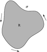
Green's theorem says
![]()
But the double integral on the right is 0, because ![]() . Therefore, the integral around a
closed curve is 0, and that is statement 3.
. Therefore, the integral around a
closed curve is 0, and that is statement 3.
Before I do the next step, here is some notation. If ![]() is a curve,
is a curve, ![]() will denote the
same curve traversed in the opposite direction.
will denote the
same curve traversed in the opposite direction.
If I traverse a curve backward, the line integral flips its sign:
![]()
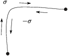
Now assume statement 3 is true: The line integral around a closed
curve is 0. Take curves ![]() and
and ![]() , both of which start at P and both of which end at
Q. I need to show that
, both of which start at P and both of which end at
Q. I need to show that
![]()

If I go from P to Q along ![]() then back from Q to P
along
then back from Q to P
along ![]() , I have a closed curve. So the integral
around
, I have a closed curve. So the integral
around ![]() is 0:
is 0:
![]()
Do each path separately:
![]()
The second integral is the negative of the integral along ![]() :
:
![]()
Finally, move the second integral to the other side:
![]()
This is what I wanted to prove, so statement 4 follows from statement 3.
Finally, suppose statement 4 is true: The field is path independent.
I want to show that ![]() is a
gradient field. I need to find a function f such that
is a
gradient field. I need to find a function f such that ![]() . To do this, take any path
. To do this, take any path ![]() from
from ![]() to
to ![]() and define
and define
![]()
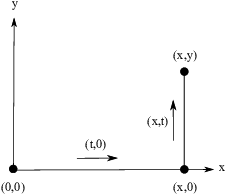
By path independence, it does not matter what path I choose, so I'll
use the path from ![]() to
to ![]() to
to ![]() made up of two segments as
shown below:
made up of two segments as
shown below:
Having defined f using this path, I have to show that ![]() and
and ![]() .
.
The horizontal part is ![]() for
for
![]() . The velocity vector is
. The velocity vector is ![]() , and
, and ![]() . So
. So
![]()
Therefore, the integral for the horizontal segment is
![]()
The vertical part is ![]() for
for ![]() . The velocity vector is
. The velocity vector is ![]() and
and ![]() . So
. So
![]()
Therefore, the integral for the vertical segment is
![]()
The line integral along the whole path --- which by definition is f --- is
![]()
Remember that I was trying to show that ![]() and
and ![]() .
Differentiate the last equation with respect to y.
.
Differentiate the last equation with respect to y.
![]()
The first integral only involves x, so its derivative with respect to
y is 0. For the second integral, apply the Fundamental Theorem of
Calculus: The y in the top limit replaces the t in the integrand and
I get ![]() . So
. So
![]()
That is, f has the right y derivative.
If you take a path made up of two segments going from ![]() to
to ![]() to
to ![]() --- along the y-axis, then horizontally --- you can
show in similar fashion that
--- along the y-axis, then horizontally --- you can
show in similar fashion that ![]() . (Remember
that I get the same "f" regardless of which path I take.)
Thus,
. (Remember
that I get the same "f" regardless of which path I take.)
Thus,
![]()
This proves statement 1.
And that finishes the proof that the four statements are equivalent.
By the way, the last part of the proof gives a way of constructing a
potential function for a gradient field. It's perhaps not the best
way for a human being to do this, but would be a reasonable approach
if you were doing this on a computer.![]()
Example. Find a potential function for ![]() using the line integrals in
the proof of the theorem.
using the line integrals in
the proof of the theorem.
I can find f using the formula
![]()
Here ![]() , so
, so ![]() . Likewise,
. Likewise,
![]() , so
, so ![]() . So
. So
![]()
By the way, notice that ![]() is also a
potential function for this field, since
is also a
potential function for this field, since ![]() and
and ![]() . There
are infinitely many potential functions for a gradient field; they
differ by a numerical constant.
. There
are infinitely many potential functions for a gradient field; they
differ by a numerical constant.![]()
So far, I've discussed vector fields in ![]() , that is, 2 dimensions. There are few surprises when
you move up to 3 dimensions.
, that is, 2 dimensions. There are few surprises when
you move up to 3 dimensions.
Theorem. Let ![]() be a 3-dimensional vector field,
and assume its components have continuous partial derivatives. Then
the following four statements are equivalent:
be a 3-dimensional vector field,
and assume its components have continuous partial derivatives. Then
the following four statements are equivalent:
1. ![]() for some function
for some function ![]() .
.
2. ![]() .
.
3. If ![]() is a closed curve ---
i.e. a path which starts and ends at the same point --- then
is a closed curve ---
i.e. a path which starts and ends at the same point --- then
![]()
4. ( Path independence) If ![]() and
and ![]() are paths which start
at the same point and end at the same point, then
are paths which start
at the same point and end at the same point, then
![]()
Once again, a field that satisfies any one of these conditions is a conservative field --- or sometimes a gradient field, or sometimes path independent.
The only change in moving from 2 dimensions to 3 dimensions is in
statement 2. To see how this is related to the ![]() for a 2-dimensional field, take a
field
for a 2-dimensional field, take a
field ![]() and regard it as a
3-dimensional field by making the third component 0, so
and regard it as a
3-dimensional field by making the third component 0, so
![]()
Then
(Notice that, e.g., ![]() , because P
does not contain any z's.) The condition
, because P
does not contain any z's.) The condition ![]() is, in this case, the same as
is, in this case, the same as ![]() .
.
In fact, the components of ![]() should have
continuous first partials, except perhaps at finitely many
points. Here's the reason I can allow finitely many "bad
points" in this case but none in the 2-dimensional case.
should have
continuous first partials, except perhaps at finitely many
points. Here's the reason I can allow finitely many "bad
points" in this case but none in the 2-dimensional case.
Think of a closed curve as a piece of string. In a rough sense, the reason why the integral of a conservative field around a closed curve is 0 is that the string can be "reeled in" to the basepoint without changing the integral.
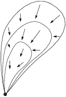
When the curve has been reeled in to a single point, the integral over the curve is obviously 0.
In 2 dimensions, a curve can "get stuck" on a single bad point as you reel it in.
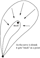
However, if the picture above is in 3 dimensions, you can "lift" the curve up out of the plane and over the point in the middle, so the curve doesn't get stuck as you reel it in.
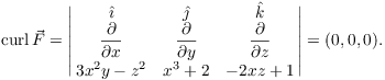
Example. Show that ![]() is
conservative, and find a potential function for
is
conservative, and find a potential function for ![]() .
.
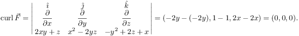
Therefore, ![]() is conservative. A potential
function f must satisfy
is conservative. A potential
function f must satisfy
![]()
Integrate the first equation with respect to x:
![]()
Since the integral is with respect to x, y and z are constant, and
must be included in the arbitrary constant ![]() . Now differentiate with respect to y and set the
result equal to
. Now differentiate with respect to y and set the
result equal to ![]() above:
above:
![]()
I find that ![]() , so integrating with
respect to y,
, so integrating with
respect to y,
![]()
This time, z is constant and must be included in the arbitrary
constant ![]() . Plug this back into f; it is
. Plug this back into f; it is
![]()
Finally, differentiate with respect to z and set the result equal to
![]() above:
above:
![]()
I find that ![]() , so
, so ![]() , where E is a numerical constant. As in an
earlier example, I may take
, where E is a numerical constant. As in an
earlier example, I may take ![]() . This gives
. This gives ![]() , so
, so
![]()
Example. Compute ![]() , where
, where
![]()
You could compute the integral directly --- would you want to? There must be an easier way ...
Since ![]() , the field is
conservative. If I can find a potential function, I can compute the
integral by simply plugging the endpoints of the path into the
potential function.
, the field is
conservative. If I can find a potential function, I can compute the
integral by simply plugging the endpoints of the path into the
potential function.
A potential function f must satisfy
![]()
Integrate the first equation with respect to x:
![]()
Since the integral is with respect to x, y and z are constant, and
must be included in the arbitrary constant ![]() . Now differentiate with respect to y and set the
result equal to
. Now differentiate with respect to y and set the
result equal to ![]() above:
above:
![]()
I find that ![]() , so integrating with respect
to y,
, so integrating with respect
to y,
![]()
This time, z is constant and must be included in the arbitrary
constant ![]() . Plug this back into f; it is
. Plug this back into f; it is
![]()
Finally, differentiate with respect to z and set the result equal to
![]() above:
above:
![]()
I find that ![]() , so
, so ![]() , where E is a numerical constant. As in an earlier
example, I may take
, where E is a numerical constant. As in an earlier
example, I may take ![]() . This gives
. This gives ![]() , so
, so
![]()
The endpoints of the path are
![]()
Therefore,
![]()
Example. ![]() is a path with
positive components from a point P on
is a path with
positive components from a point P on ![]() to a point Q on
to a point Q on ![]() . Compute
. Compute ![]() , where
, where
![]()
The path isn't given --- in fact, its endpoints aren't given.
Therefore, the path must not matter, i.e. the integral is
probably path independent. In fact, ![]() , for
, for ![]() .
Therefore,
.
Therefore,
![]()
Now Q is on ![]() , so for this point
, so for this point ![]() . Likewise, P is on
. Likewise, P is on ![]() , so for this point
, so for this point ![]() . Hence,
. Hence,
![]()
Copyright 2022 by Bruce Ikenaga