In this section, we'll derive some properties of determinants. Two key results: The determinant of a matrix is equal to the determinant of its transpose, and the determinant of a product of two matrices is equal to the product of their determinants.
We'll also derive a formula involving the adjugate of a matrix. We'll use it to give a formula for the inverse of a matrix, and to derive Cramer's rule, a method for solving some systems of linear equations.
The first result is a corollary of the permutation formula for determinants which we derived earlier.
Corollary. Let R be a commutative ring with
identity, and let ![]() . Then
. Then ![]() .
.
Proof. We'll use the permutation formula for
the determinant, beginning with the determinant of ![]() .
.
![]()
![]()
![]()
In the fourth equality, I went from summing over ![]() in
in ![]() to
to ![]() in
in ![]() . This is valid
because permutations are bijective functions, so they have inverse
functions which are also permutations. So summing over all
permutations in
. This is valid
because permutations are bijective functions, so they have inverse
functions which are also permutations. So summing over all
permutations in ![]() is the same as summing over all
their inverses in
is the same as summing over all
their inverses in ![]() --- you will get the
same terms in the sum, just in a different order.
--- you will get the
same terms in the sum, just in a different order.
I got the next-to-the-last equality by letting ![]() . This just makes it easier to
recognize the next-to-last expression as the permutation formula for
. This just makes it easier to
recognize the next-to-last expression as the permutation formula for
![]() .
.![]()
Remark. We've used row operations as an aid to
computing determinants. Since the rows of A are the columns of ![]() and vice versa, the Corollary implies that you can
also use column operations to compute determinants. The allowable
operations are swapping two columns, multiplying a column by a
number, and adding a multiple of a column to another column. They
have the same effects on the determinant as the corresponding row
operations.
and vice versa, the Corollary implies that you can
also use column operations to compute determinants. The allowable
operations are swapping two columns, multiplying a column by a
number, and adding a multiple of a column to another column. They
have the same effects on the determinant as the corresponding row
operations.
This also means that you can compute determinants using cofactors of rows as well as columns.
In proving the uniqueness of determinant functions, we showed that if
D is a function on ![]() matrices which is
alternating and linear on the rows, then
matrices which is
alternating and linear on the rows, then ![]() . We will use this to prove the
product rule for determinants.
. We will use this to prove the
product rule for determinants.
Theorem. Let R be a commutative ring with
identity, and let ![]() . Then
. Then ![]() .
.
Proof. Fix B, and define
![]()
I will show that D is alternating and linear, then apply a result I derived in showing uniqueness of determinant functions.
Let ![]() denote the i-th row of A. Then
denote the i-th row of A. Then

Now ![]() is alternating, so interchanging two rows
in the determinant above multiplies
is alternating, so interchanging two rows
in the determinant above multiplies ![]() by -1. Hence, D is alternating.
by -1. Hence, D is alternating.
Next, I'll show that D is linear:
![$$D\left[\matrix{ & \vdots & \cr \leftarrow & k x + y & \rightarrow \cr & \vdots & \cr}\right] = \left|\matrix{ & \vdots & \cr \leftarrow & (k x + y) B & \rightarrow \cr & \vdots & \cr}\right| =$$](determinants-properties25.png)
![$$k \cdot \left|\matrix{ & \vdots & \cr \leftarrow & x B & \rightarrow \cr & \vdots & \cr}\right| + \left|\matrix{& \vdots & \cr \leftarrow & yB & \rightarrow \cr & \vdots & \cr}\right| = k \cdot D\left[\matrix{ & \vdots & \cr \leftarrow & x & \rightarrow \cr & \vdots & \cr}\right] + D\left[\matrix{ & \vdots & \cr \leftarrow & y & \rightarrow \cr & \vdots & \cr}\right].$$](determinants-properties26.png)
This proves that D is linear in each row.
Since D is a function on ![]() which is
alternating and linear in the rows, the result I mentioned earlier
shows
which is
alternating and linear in the rows, the result I mentioned earlier
shows
![]()
But ![]() and
and ![]() , so we get
, so we get
![]()
In other words, the determinant of a product is the product of the determinants. A similar result holds for powers.
Corollary. Let R be a commutative ring with
identity, and let ![]() . Then for every
. Then for every
![]() ,
,
![]()
Proof. This follows from the previous result
using induction. The result is obvious for ![]() and
and ![]() (note that
(note that ![]() , the identity matrix), and the case
, the identity matrix), and the case ![]() follows from the previous result if we take
follows from the previous result if we take ![]() .
.
Suppose the result is true for m, so ![]() . We need to show that the result holds for
. We need to show that the result holds for
![]() . We have
. We have
![]()
We used the case ![]() to get the second equality,
and the induction assumption was used to get the third equality. This
proves the result for
to get the second equality,
and the induction assumption was used to get the third equality. This
proves the result for ![]() , so it holds for
all
, so it holds for
all ![]() by induction.
by induction.![]()
While the determinant of a product is the product of the determinants, the determinant of a sum is not necessarily the sum of the determinants.
Example. Give a specific example of ![]() real matrices A and B for which
real matrices A and B for which ![]() .
.
![]()
But
![]()
The rule for products gives us an easy criterion for the invertibility of a matrix. First, I'll prove the result in the special case where the entries of the matrix are elements of a field.
Theorem. Let F be a field, and let ![]() .
.
A is invertible if and only if ![]() .
.
Proof. If A is invertible, then
![]()
This equation implies that ![]() (since
(since ![]() would yield "
would yield "![]() ").
").
Conversely, suppose that ![]() . Suppose that A
row reduces to the row reduced echelon matrix R, and consider the
effect of elementary row operations on
. Suppose that A
row reduces to the row reduced echelon matrix R, and consider the
effect of elementary row operations on ![]() . Swapping two rows multiplies the determinant by -1.
Adding a multiple of a row to another row leaves the determinant
unchanged. And multiplying a row by a nonzero number
multiplies the determinant by that nonzero number. Clearly,
no row operation will make the determinant 0 if it was nonzero to
begin with. Since
. Swapping two rows multiplies the determinant by -1.
Adding a multiple of a row to another row leaves the determinant
unchanged. And multiplying a row by a nonzero number
multiplies the determinant by that nonzero number. Clearly,
no row operation will make the determinant 0 if it was nonzero to
begin with. Since ![]() , it follows that
, it follows that ![]() .
.
Since R is a row reduced echelon matrix with nonzero determinant, it
can't have any all-zero rows. An ![]() row reduced echelon matrix with no all-zero
rows must be the identity, so
row reduced echelon matrix with no all-zero
rows must be the identity, so ![]() . Since A row reduces to the identity, A is
invertible.
. Since A row reduces to the identity, A is
invertible.![]()
Corollary. Let F be a field, and let ![]() . If A is invertible, then
. If A is invertible, then
![]()
Proof. I showed in proving the theorem that
![]() , so
, so ![]() .
.![]()
We'll see below what happens if we have a commutative ring with identity instead of a field.
The next example uses the determinant properties we've derived.
Example. Suppose A, B, and C are ![]() matrices over
matrices over ![]() , and
, and
![]()
Compute ![]() .
.
We have ![]() and
and ![]() . Using the
product rule for determinants,
. Using the
product rule for determinants,
![]()
Definition. Let R be a commutative ring with
identity. Matrices ![]() are similar if there is an invertible matrix
are similar if there is an invertible matrix ![]() such that
such that ![]() .
.
Similar matrices come up in many places, for instance in changing bases for vector spaces.
Corollary. Let R be a commutative ring with
identity. Similar matrices in ![]() have equal determinants.
have equal determinants.
Proof. Suppose A and B are similar, so ![]() for some invertible matrix P. Then
for some invertible matrix P. Then
![]()
In the third equality, I used the fact that ![]() and
and ![]() are numbers --- elements of the ring R ---
and multiplication in R is commutative. That allows me to commute
are numbers --- elements of the ring R ---
and multiplication in R is commutative. That allows me to commute
![]() and
and ![]() .
.![]()
Definition. Let R be a commutative ring with
identity, and let ![]() . The adjugate
. The adjugate ![]() is the matrix whose
i-j-th entry is
is the matrix whose
i-j-th entry is
![]()
In other words, ![]() is the transpose of the matrix
of cofactors.
is the transpose of the matrix
of cofactors.
Remark. In the past, ![]() was referred to as the
adjoint, or the classical adjoint. But
the term "adjoint" is now used to refer to something else:
The conjugate transpose, which we'll see when
we discuss the spectral theorem. So the term
"adjugate" has come to replace it for the matrix defined
above. One advantage of the word "adjugate" is that you can
use the same abbreviation "adj" as was used for
"adjoint"!
was referred to as the
adjoint, or the classical adjoint. But
the term "adjoint" is now used to refer to something else:
The conjugate transpose, which we'll see when
we discuss the spectral theorem. So the term
"adjugate" has come to replace it for the matrix defined
above. One advantage of the word "adjugate" is that you can
use the same abbreviation "adj" as was used for
"adjoint"!
Example. Compute the adjugate of
![$$A = \left[\matrix{ 1 & 0 & 3 \cr 0 & 1 & 1 \cr 1 & -1 & 2 \cr}\right].$$](determinants-properties88.png)
First, I'll compute the cofactors. The first line shows the cofactors of the first row, the second line the cofactors of the second row, and the third line the cofactors of the third row.
![]()
![]()
![]()
The adjugate is the transpose of the matrix of cofactors:
![$$\adj A = \left[\matrix{ 3 & -3 & -3 \cr 1 & -1 & -1 \cr -1 & 1 & 1 \cr}\right].\quad\halmos$$](determinants-properties92.png)
The next result shows that adjugates and tranposes can be interchanged: The adjugate of the transpose equals the transpose of the adjugate.
Proposition. Let R be a commutative ring with
identity, and let ![]() . Then
. Then
![]()
Proof. Consider the ![]() elements of the matrices on the two sides
of the equation.
elements of the matrices on the two sides
of the equation.
![]()
![]()
The signs ![]() and
and ![]() are the same; what about the other terms?
are the same; what about the other terms?
![]() is the determinant of the matrix
formed by deleting the
is the determinant of the matrix
formed by deleting the ![]() row and the
row and the
![]() column from A. And
column from A. And ![]() is the determinant of the matrix formed by
deleting the
is the determinant of the matrix formed by
deleting the ![]() row and
row and ![]() column from
column from ![]() . But the
. But the ![]() row of A is the
row of A is the
![]() column of
column of ![]() , and the
, and the ![]() column of A is
the
column of A is
the ![]() row of
row of ![]() . So the two matrices that remain after these
deletions are transposes of one another, and hence they have the same
determinant. Thus,
. So the two matrices that remain after these
deletions are transposes of one another, and hence they have the same
determinant. Thus, ![]() . Hence,
. Hence, ![]() .
.![]()
The next theorem is very important, but the proof is a little tricky. So I'll discuss the main point in the proof first by giving an example.
Suppose we compute the following determinant over ![]() using expansion by cofactors on the
using expansion by cofactors on the ![]() row:
row:

![]()
As usual, I multiplied the cofactors of the ![]() row by the elements of the
row by the elements of the ![]() row.
row.
Now suppose I make a mistake: I multiply the cofactors of the ![]() row by elements of the
row by elements of the ![]() row (which are 1, 2, 4). Here's what I get:
row (which are 1, 2, 4). Here's what I get:
![]()
![]()
Or suppose I multiply the cofactors of the ![]() row by elements of the
row by elements of the ![]() row (which are 1, -1, 0). Here's what I
get:
row (which are 1, -1, 0). Here's what I
get:
![]()
![]()
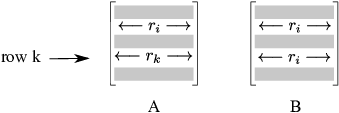
These examples suggest that if I try to do a cofactor expansion by using the cofactors of one row multiplied by the elements from another row, I get 0. It turns out that this is true in general, and is the key step in the next proof.
Theorem. Let R be a commutative ring with
identity, and let ![]() . Then
. Then
![]()
Proof. This proof is a little tricky, so you may want to skip it for now.
We expand ![]() by cofactors of row i:
by cofactors of row i:
![]()
First, suppose ![]() . Construct a new matrix B by
replacing row k of A with row i of A. Thus, the elements of B are the
same as those of A, except that B's row k duplicates A's row i.
. Construct a new matrix B by
replacing row k of A with row i of A. Thus, the elements of B are the
same as those of A, except that B's row k duplicates A's row i.
In symbols,
![]()
Suppose we compute ![]() by expanding by
cofactors of row k. We get
by expanding by
cofactors of row k. We get
![]()
Why is ![]() ? To compute
? To compute
![]() , you delete row k and column j
from B. To compute
, you delete row k and column j
from B. To compute ![]() , you delete
row k and column j from A. But A and B only differ in row k, which is
being deleted in both cases. Hence,
, you delete
row k and column j from A. But A and B only differ in row k, which is
being deleted in both cases. Hence, ![]() .
.

On the other hand, B has two equal rows --- its row i and row k are both equal to row i of A --- so the determinant of B is 0. Hence,
![]()
This is the point we illustrated prior to stating the theorem: if you
do a cofactor expansion by using the cofactors of one row multiplied
by the elements from another row, you get 0. The last equation is
what we get for ![]() . In case
. In case ![]() , we just get the cofactor expansion for
, we just get the cofactor expansion for ![]() :
:
![]()
We can combine the two equations into one using the Kronecker delta function:
![]()
Remember that ![]() if
if ![]() , and
, and ![]() if
if ![]() . These are the two cases above.
. These are the two cases above.
Interpret this equation as a matrix equation, where the two sides
represent the ![]() -th entries of their
respective matrices. What are the respective matrices? Since
-th entries of their
respective matrices. What are the respective matrices? Since
![]() is the
is the ![]() -th entry of the identity matrix, the right
side is the
-th entry of the identity matrix, the right
side is the ![]() -th entry of
-th entry of ![]() .
.
The left side is the ![]() -th entry of
-th entry of ![]() , because
, because
![]()
Therefore,
![]()
I can use the theorem to obtain an important corollary. I already know that a matrix over a field is invertible if and only if its determinant is nonzero. The next result explains what happens over a commutative ring with identity, and also provides a formula for the inverse of a matrix.
Corollary. Let R be a commutative ring with
identity. A matrix ![]() is invertible if and
only if
is invertible if and
only if ![]() is invertible in R, in which case
is invertible in R, in which case
![]()
Proof. First, suppose A is invertible. Then
![]() , so
, so
![]()
Therefore, ![]() is invertible in R.
is invertible in R.
Since ![]() is invertible, I can take the equation
is invertible, I can take the equation ![]() and multiply by
and multiply by ![]() to get
to get
![]()
This implies that ![]() .
.
Conversely, suppose ![]() is invertible in R. As
before, I get
is invertible in R. As
before, I get
![]()
Again, this implies that ![]() , so A is invertible.
, so A is invertible.![]()
As a special case, we get the formula for the inverse of a ![]() matrix.
matrix.
Corollary. Let R be a commutative ring with
identity. Suppose ![]() , and
, and ![]() is invertible in R. Then
is invertible in R. Then
![]()
Proof.
![]()
Hence, the result follows from the adjugate formula.![]()
To see the difference between the general case of a commutative ring
with identity and a field, consider the following matrices over ![]() :
:
![]()
In the first case,
![]()
2 is not invertible in ![]() --- do you know
how to prove it? Hence, even though the determinant is nonzero, the
matrix is not invertible.
--- do you know
how to prove it? Hence, even though the determinant is nonzero, the
matrix is not invertible.
![]()
5 is invertible in ![]() --- in fact,
--- in fact,
![]() . Hence, the second matrix is
invertible. You can find the inverse using the formula in the last
corollary.
. Hence, the second matrix is
invertible. You can find the inverse using the formula in the last
corollary.
The adjugate formula can be used to find the inverse of a matrix.
It's not very good for big matrices from a computational point of
view: The usual row reduction algorithm uses fewer steps. However,
it's not too bad for small matrices --- say ![]() or smaller.
or smaller.
Example. Compute the inverse of the following real matrix using the adjugate formula.
![$$A = \left[\matrix{ 1 & -2 & -2 \cr 3 & -2 & 0 \cr 1 & 1 & 1 \cr}\right].$$](determinants-properties189.png)
First, I'll compute the cofactors. The first line shows the cofactors of the first row, the second line the cofactors of the second row, and the third line the cofactors of the third row. I'm showing the "checkerboard" pattern of pluses and minuses as well.
![]()
![]()
![]()
The adjugate is the transpose of the matrix of cofactors:
![$$\adj A = \left[\matrix{ -2 & 0 & -4 \cr -3 & 3 & -6 \cr 5 & -3 & 4 \cr}\right].$$](determinants-properties193.png)
I'll let you show that ![]() . So I have
. So I have
![$$A^{-1} = -\dfrac{1}{6} \left[\matrix{ -2 & 0 & -4 \cr -3 & 3 & -6 \cr 5 & -3 & 4 \cr}\right].\quad\halmos$$](determinants-properties195.png)
Another consequence of the formula ![]() is Cramer's
rule, which gives a formula for the solution of a system of
linear equations.
is Cramer's
rule, which gives a formula for the solution of a system of
linear equations.
Corollary. ( Cramer's
rule) If A is an invertible ![]() matrix, the unique solution to
matrix, the unique solution to ![]() is given by
is given by
![]()
Here ![]() is the matrix obtained from A by replacing
its i-th column by y.
is the matrix obtained from A by replacing
its i-th column by y.
Proof.
![]()
Hence,
![]()
But the last sum is a cofactor expansion of A along column i, where
instead of the elements of A's column i I'm using the components of
y. This is exactly ![]() .
.![]()
Example. Use Cramer's Rule to solve the
following system over ![]() :
:

In matrix form, this is
![$$\left[\matrix{ 2 & 1 & 1 \cr 1 & 1 & -1 \cr 3 & -1 & 2 \cr}\right] \left[\matrix{x \cr y \cr z \cr}\right] = \left[\matrix{1 \cr 5 \cr -2 \cr}\right].$$](determinants-properties206.png)
I replace the successive columns of the coefficient matrix with ![]() , in each case computing the determinant of
the resulting matrix and dividing by the determinant of the
coefficient matrix:
, in each case computing the determinant of
the resulting matrix and dividing by the determinant of the
coefficient matrix:

This looks pretty simple, doesn't it? But notice that you need to
compute four ![]() determinants to
do this (and I didn't write out the work for those computations!). It
becomes more expensive to solve systems this way as the matrices get
larger.
determinants to
do this (and I didn't write out the work for those computations!). It
becomes more expensive to solve systems this way as the matrices get
larger.![]()
As with the adjugate formula for the inverse of a matrix, Cramer's rule is not computationally efficient: It's better to use row reduction to solve large systems. Cramer's rule is not too bad for solving systems of two linear equations in two variables; for anything larger, you're probably better off using row reduction.
Copyright 2022 by Bruce Ikenaga