Imagine a thin piece of wire, which only gains or loses heat through
its ends. The temperature ![]() is a function of the position x
along the wire and the time t. It is a solution to the heat equation
is a function of the position x
along the wire and the time t. It is a solution to the heat equation
![]()
The solution to the one-dimensional heat equation with an arbitrary initial distribution is an infinite sum
![]()
If ![]() is the initial distribution, then the
is the initial distribution, then the ![]() 's
are given by
's
are given by
![]()
That is, ![]() is expressed as an infinite sum of sines.
is expressed as an infinite sum of sines.
A Fourier series represents a function ![]() as
an infinite sum of trigonometric functions:
as
an infinite sum of trigonometric functions:
![]()
Consider integrable functions f and g defined on the interval ![]() , where
, where ![]() . Define the
inner product of f and g by
. Define the
inner product of f and g by
![]()
Example. Verify the linearity and symmetry axioms for an inner product for
![]()
Let ![]() and
and ![]() and
and ![]() be integrable functions on
be integrable functions on ![]() . Using properties of integrals, I have
. Using properties of integrals, I have
![]()
![]()
Symmetry is easy:
![]()
Note that this should be called "inner product" (with
quotes), since it isn't positive definite. Since ![]() , it follows that
, it follows that
![]()
But you could have a function which was nonzero --- for example, a
function which was 0 at every point in ![]() , but
nonzero at a single point --- such that
, but
nonzero at a single point --- such that ![]() .
.
We can get around this problem by confining ourselves to continuous functions. Unfortunately, many of the
functions we'd like to apply Fourier series to aren't continuous.![]()
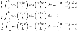
Theorem. ( Orthogonality Relations)
Example. I'll illustrate the first formula with some numerical examples.
If I take different cosines, I should get 0. I'll try
![]()
Use the identity
![]()
I get
![]()
So
![]()
![]()
(Remember that the sine of a multiple of ![]() is 0!)
is 0!)
If I do the integral with both cosines the same, I use the double angle formula:
![]()
![]()
There is nothing essentially different in the derivation of the
general formulas.![]()
In terms of the (almost) inner product defined above, the orthogonality relations are:
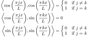
In other words, the sine and cosine functions form an orthnormal set (again, allowing that we don't quite have an inner product here).
As a constant function, I'll use ![]() . You
can verify that this is perpendicular to the sines and cosines above,
and that it has length 1.
. You
can verify that this is perpendicular to the sines and cosines above,
and that it has length 1.
For vectors in an inner product space, you can get the components of
a vectors by taking the inner product of the vector with elements of
an orthonormal basis. For example, if ![]() is an orthonormal basis, then a vector x can be written as a linear
combination of the u's by taking inner product of x with the u's:
is an orthonormal basis, then a vector x can be written as a linear
combination of the u's by taking inner product of x with the u's:
![]()
By analogy, I might try to expand a function in terms of the sines
and cosines by taking the inner product of f with the sines and
cosines, and the constant function ![]() .
Doing so, I get
.
Doing so, I get
![]()
![]()
The cosine term is ![]() .
.
The sine term is ![]() .
.
If I set ![]() in the
in the ![]() formula, then since
formula, then since ![]() , I'd get
, I'd get
![]()
So for the constant function ![]() , the
coefficient is
, the
coefficient is
![]()
But my constant function is ![]() , so
the constant term in the series will be
, so
the constant term in the series will be
![]()
Putting everything together gives the Fourier series for ![]() :
:
![]()
You can interpret it as an expression for f as an infinite "linear combination" of the orthnormal sine and cosine functions.
There are several issues here. For one thing, this is an infinite
sum, not the usual finite linear combination which expresses
a vector in terms of a basis. Questions of convergence always arise
with infinite sums. Moreover, even if the infinite sum converges, why
should it converge to ![]() ?
?
In addition, we're only doing this by analogy with our results on inner product spaces, because this "inner product" only satisfies two of the inner product axioms.
It's important to know that these issues exist, but their treatment will be deferred to an advanced course in analysis.
Before doing some examples, here are some notes about computations.
You can often use the complex exponential (DeMoivre's formula) to simplify computations:
![]()
Specifically, let
![]()
Then
![]()
This allows me to compute a single integral, then find the real and imaginary parts of the result to get the sine and cosine coefficients.
On some occasions, symmetry can be used to obtain the values of some of the coefficients.
1. If a function is even --- that is, if ![]() for all x, so the graph is symmetric about the y-axis
--- then
for all x, so the graph is symmetric about the y-axis
--- then ![]() for all n.
for all n.
2. If a function is odd --- that is, if ![]() for all x, so the graph is symmetric about the origin
--- then
for all x, so the graph is symmetric about the origin
--- then ![]() for all n.
for all n.
This makes sense, since the cosine functions are even and the sine functions are odd.
Here's a final remark before I get to the examples. A sum of periodic
functions is periodic. Since sine and cosine are periodic, you can
only expect to represent periodic functions by a Fourier series.
Therefore, outside the interval ![]() , you must
"repeat"
, you must
"repeat" ![]() in periodic fashion (so
in periodic fashion (so ![]() for all x).
for all x).
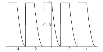
For example, consider the function ![]() ,
, ![]() .
. ![]() , so I must "repeat" the function
every two units. Picture:
, so I must "repeat" the function
every two units. Picture:
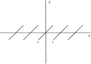
The Fourier expansion of ![]() only converges to
only converges to ![]() on the interval
on the interval ![]() . Outside of that interval, it converges to
the periodic function in the picture (except perhaps at the jump
discontinuities).
. Outside of that interval, it converges to
the periodic function in the picture (except perhaps at the jump
discontinuities).
Example. Find the Fourier expansion of
![]()
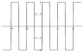
This graph is called a square wave.
This is an odd function, so ![]() for all k --- that is, all the
cosine terms vanish. I'll compute all the coefficients anyway so you
can see this directly.
for all k --- that is, all the
cosine terms vanish. I'll compute all the coefficients anyway so you
can see this directly.
Compute the constant term first:
![]()
Next, compute the ![]() terms:
terms:
![]()
![]()
Now
![]()
![]()
So
![]()
Now
![]()
So the Fourier expansion is
![]()
Here are the graphs of the first, fifth, and tenth partial sums:
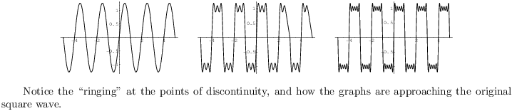
Note that if ![]() , all the terms of the series are 0, and
the series converges to 0. In fact, under reasonable conditions ---
specifically, if f is of bounded variation in
an interval around a point c --- the Fourier series will converges to
the average of the left and right-hand limits at the point. In this
case, the left-hand limit is -1, the right-hand limit is 1, and their
average is 0. On the other hand,
, all the terms of the series are 0, and
the series converges to 0. In fact, under reasonable conditions ---
specifically, if f is of bounded variation in
an interval around a point c --- the Fourier series will converges to
the average of the left and right-hand limits at the point. In this
case, the left-hand limit is -1, the right-hand limit is 1, and their
average is 0. On the other hand, ![]() was defined to be
1.
was defined to be
1.![]()
Example. Find the Fourier expansion of
![]()
Compute the constant term first:
![]()
Next, compute the higher order terms:
![]()
![]()
![]()
Therefore,
![]()
![]()
Now take real and imaginary parts:
![]()
The Fourier series is
![]()
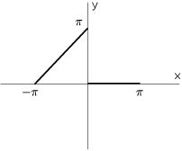
Example. Find the Fourier expansion of
![]()
Compute the constant term first:
![]()
Next, compute the higher order terms. As in the computation of ![]() ,
I only need the integral from
,
I only need the integral from ![]() to 0, since the function equals 0
from 0 to
to 0, since the function equals 0
from 0 to ![]() :
:
![]()
![]()
![]()
Thus,
![]()
The series is
![]()
Copyright 2016 by Bruce Ikenaga