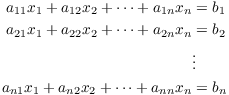
Matrix inversion gives a method for solving some systems of equations. Suppose we have a system of n linear equations in n variables:
Let
![$$A = \left[\matrix{a_{11} & a_{12} & \ldots & a_{1n} \cr a_{21} & a_{22} & \ldots & a_{2n} \cr \vdots & \vdots & \ddots & \vdots \cr a_{n1} & a_{n2} & \ldots & a_{nn} \cr}\right], \quad x = \left[\matrix{x_1 \cr x_2 \cr \vdots \cr x_n \cr}\right], \quad b = \left[\matrix{b_1 \cr b_2 \cr \vdots \cr b_n \cr}\right].$$](inverses-and-elementary-matrices2.png)
The system can then be written in matrix form:
![]()
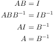
(One reason for using matrix notation is that it saves writing!) If A
has an inverse ![]() , I can multiply
both sides by
, I can multiply
both sides by ![]() :
:
I've solved for the vector x of variables.
Not every matrix has an inverse --- an obvious example is the zero matrix, but here's a nonzero non-invertible matrix over the real numbers:
![]()
Suppose this matrix had an inverse ![]() . Then
. Then
![]()
But equating entries in row 2, column 2 gives the contradiction ![]() . Hence, the original matrix does not have
an inverse.
. Hence, the original matrix does not have
an inverse.
If we want to know whether a matrix has an inverse, we could try to do what we did in this example --- set up equations and see if we can solve them. But you can see that it could be pretty tedious if the matrix was large or the entries were messy. And we saw earlier that you can solve systems of linear equations using row reduction.
In this section, we'll see how you can use row reduction to determine whether a matrix has an inverse --- and, if it does, how to find the inverse. We'll begin by explaining the connection between elementary row operations and matrices.
Definition. An elementary matrix is a matrix which represents an elementary row operation. "Represents" means that multiplying on the left by the elementary matrix performs the row operation.
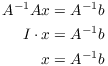
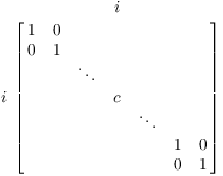
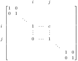
Here are the elementary matrices that represent our three types of row operations. In the pictures below, the elements that are not shown are the same as those in the identity matrix. In particular, all of the elements that are not on the main diagonal are 0, and all the main diagonal entries --- except those shown --- are 1.
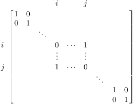
Multiplying by this matrix swaps rows i and j:

The "i" and "j" on the borders of the matrix label rows and columns so you can see where the elements are.
This is the same as the identity matrix, except that rows i and j have been swapped. In fact, you obtain this matrix by applying the row operation ("swap rows i and j") to the identity matrix. This is true for our other elementary matrices.
Multiplying by this matrix multiplies row i by the number c:
This is the same as the identity matrix, except that row i has been multiplied by c. Note that this is only a valid operation if the number c has a multiplicative inverse. For instance, if we're working over the real numbers, c can be any nonzero number.
Multiplying by this matrix replaces row i with row i plus c times row j.
To get this matrix, apply the operation "add c times row j to row i" to the identity matrix.
While we could give formal proofs that these matrices do what we want --- we would have to write formulas for elements of the matrices, then use the definition of matrix multiplication --- I don't think the proofs would be very enlightening. It's good, however, to visualize the multiplications for yourself to see why these matrices work: Take rows of the elementary matrix and picture them multiplying rows of the original matrix. For example, consider the elementary matrix that swaps row i and row j.
When you multiply the original matrix by row FOO of this matrix, you get row FOO of the product. So multiplying the original matrix by first row of this matrix gives the first row of the product, and so on. Let's look at what happens when you multiply the original matrix by row i of this matrix.
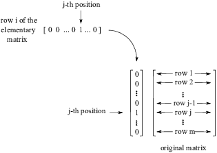
Row i has 0's everywhere except for a 1 in the ![]() position. So when it multiplies
the original matrix, all the rows of the original matrix get
multiplied by 0, except for the
position. So when it multiplies
the original matrix, all the rows of the original matrix get
multiplied by 0, except for the ![]() row, which is multiplied by 1. The
net result is the
row, which is multiplied by 1. The
net result is the ![]() row of the
original matrix. Thus, the
row of the
original matrix. Thus, the ![]() row of the product is the
row of the product is the ![]() row of the original matrix.
row of the original matrix.
If you picture this process one row at a time, you'll see that the original matrix is replaced with the same matrix with the i and j rows swapped.
Let's try some examples.
This elementary matrix should swap rows 2 and 3 in a ![]() matrix:
matrix:
![$$\left[\matrix{ 1 & 0 & 0 \cr 0 & 0 & 1 \cr 0 & 1 & 0 \cr}\right]$$](inverses-and-elementary-matrices22.png)
Notice that it's the identity matrix with rows 2 and 3 swapped.
Multiply a ![]() matrix by it on the
left:
matrix by it on the
left:
![$$\left[\matrix{ 1 & 0 & 0 \cr 0 & 0 & 1 \cr 0 & 1 & 0 \cr}\right] \left[\matrix{ a & b & c \cr d & e & f \cr g & h & i \cr}\right] = \left[\matrix{ a & b & c \cr g & h & i \cr d & e & f \cr}\right].$$](inverses-and-elementary-matrices24.png)
Rows 2 and 3 were swapped --- it worked!
This elementary matrix should multiply row 2 of a ![]() matrix by 13:
matrix by 13:
![]()
Notice that it's the identity matrix with row 2 multiplied by 13. (We'll assume that we're in a number system where 13 is invertible.)
Multiply a ![]() matrix by it on the
left:
matrix by it on the
left:
![]()
Row 2 orf the original matrix was multiplied by 13.
This elementary matrix should add 5 times row 1 to row 3:
![$$\left[\matrix{ 1 & 0 & 0 \cr 0 & 1 & 0 \cr 5 & 0 & 1 \cr}\right]$$](inverses-and-elementary-matrices29.png)
Notice that it's the identity matrix with 5 times row 1 added to row 3.
Multiply a ![]() matrix by it on the
left:
matrix by it on the
left:
![$$\left[\matrix{ 1 & 0 & 0 \cr 0 & 1 & 0 \cr 5 & 0 & 1 \cr}\right] \left[\matrix{ a & b & c \cr d & e & f \cr g & h & i \cr}\right] = \left[\matrix{ a & b & c \cr d & e & f \cr g + 5 a & h + 5 b & i + 5 c \cr}\right].$$](inverses-and-elementary-matrices31.png)
You can see that 5 times row 1 was added to row 3.
The inverses of these matrices are, not surprisingly, the elementary matrices which represent the inverse row operations. The inverse of a row operation is the row operation which undoes the original row operation. Let's look at the three operations in turn.
The inverse of swapping rows i and j is swapping rows i and j --- to undo swapping two things, you swap the two things back! So the inverse of the "swap row i and j" elementary matrix the the same matrix:

The inverse of multiplying row i by c is dividing row i by c. To
account for the fact that a number system might not have
"division", I'll say "multiplying row i by ![]() ". Just take the original
"multiply row i by c" elementary matrix above and replace c
with
". Just take the original
"multiply row i by c" elementary matrix above and replace c
with ![]() :
:

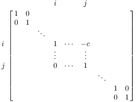
The inverse of adding c times row j to row i is subtracting c times
row j from row i. To write down the inverse, I just replace c with
![]() in the matrix for "row i goes to row i
plus c times row j":
in the matrix for "row i goes to row i
plus c times row j":
Example. In each case, tell what row operation is performed by multiplying on the left by the elementary matrix. Then find the inverse of the elementary matrix, and tell what row operation is performed by multiplying on the left by the inverse. (All the matrices are real number matrices.)
(a) ![$\displaystyle \left[\matrix{1 & 0 & 2 \cr 0 & 1 & 0 \cr 0 & 0 &
1 \cr}\right]$](inverses-and-elementary-matrices38.png)
(b) ![$\displaystyle \left[\matrix{0 & 1 & 0 \cr 1 & 0 & 0 \cr 0 & 0 &
1 \cr}\right]$](inverses-and-elementary-matrices39.png)
(c) ![$\displaystyle \left[\matrix{1 & 0 & 0 \cr 0 & 17 & 0 \cr 0 & 0
& 1 \cr}\right]$](inverses-and-elementary-matrices40.png)
(a) Multiplying on the left by
![$$\left[\matrix{1 & 0 & 2 \cr 0 & 1 & 0 \cr 0 & 0 & 1 \cr}\right] \quad\hbox{adds 2 times row 3 to row 1}.$$](inverses-and-elementary-matrices41.png)
The inverse
![$$\left[\matrix{1 & 0 & 2 \cr 0 & 1 & 0 \cr 0 & 0 & 1 \cr}\right]^{-1} = \left[\matrix{1 & 0 & -2 \cr 0 & 1 & 0 \cr 0 & 0 & 1 \cr}\right] \quad\hbox{subtracts 2 times row 3 from row 1}.$$](inverses-and-elementary-matrices42.png)
(b) Multiplying on the left by
![$$\left[\matrix{0 & 1 & 0 \cr 1 & 0 & 0 \cr 0 & 0 & 1 \cr}\right] \quad\hbox{swaps row 1 and row 2}.$$](inverses-and-elementary-matrices43.png)
The inverse
![$$\left[\matrix{0 & 1 & 0 \cr 1 & 0 & 0 \cr 0 & 0 & 1 \cr}\right]^{-1} = \left[\matrix{0 & 1 & 0 \cr 1 & 0 & 0 \cr 0 & 0 & 1 \cr}\right] \quad\hbox{swaps row 1 and row 1}.$$](inverses-and-elementary-matrices44.png)
(c) Multiplying on the left by
![$$\left[\matrix{1 & 0 & 0 \cr 0 & 17 & 0 \cr 0 & 0 & 1 \cr}\right] \quad\hbox{multiplies row 2 by 17}.$$](inverses-and-elementary-matrices45.png)
The inverse
![$$\left[\matrix{1 & 0 & 0 \cr 0 & 17 & 0 \cr 0 & 0 & 1 \cr}\right]^{-1} = \left[\matrix{1 & 0 & 0 \cr \noalign{\vskip2pt} 0 & \dfrac{1}{17} & 0 \cr \noalign{\vskip2pt} 0 & 0 & 1 \cr}\right] \quad\hbox{divides row 2 by 17}.\quad\halmos$$](inverses-and-elementary-matrices46.png)
Definition. Matrices A and B are row equivalent if A can be transformed to B by a finite sequence of elementary row operations.
Of course, row equivalent matrices must have the same dimensions.
Remark. Since row operations may be performed
by multiplying by elementary matrices, A and B are row equivalent if
and only if there are elementary matrices ![]() , ...,
, ..., ![]() such that
such that
![]()
Lemma. Row equivalence is an equivalence relation.
Proof. Let's recall what it means (in this situation) to be an equivalence relation. I have to show three things:
(a) (Reflexivity) Every matrix is row equivalent to itself.
(b) (Symmetry) If A row reduces to B, then B row reduces to A.
(c) (Transitivity) If A row reduces to B and B row reduces to C, then A row reduces to C.
(a) is obvious, since I can row reduce a matrix to itself by performing the identity row operation.
For (b), suppose A row reduces to B. Then there are elementary
matrices ![]() , ...
, ... ![]() such that
such that
![]()
Hence,
![]()
Since the inverse of an elementary matrix is an elementary matrix,
each ![]() is an elementary
matrix. This equation gives a sequence of row operations which row
reduces B to A.
is an elementary
matrix. This equation gives a sequence of row operations which row
reduces B to A.
To prove (c), suppose A row reduces to B and B row reduces to C. Then
there are elementary matrices ![]() , ...,
, ..., ![]() and
and ![]() , ...,
, ..., ![]() such that
such that
![]()
Hence,
![]()
This equation gives a sequence of row operations which row reduces A to C.
Therefore, row equivalence is an equivalence relation.![]()
Let's recall the definition of invertibility and the inverse of a matrix.
Definition. An ![]() matrix A is
invertible if there is an
matrix A is
invertible if there is an ![]() matrix B such that
matrix B such that ![]() , where I is the
, where I is the ![]() identity matrix.
identity matrix.
In this case, B is the inverse of A (or A is
the inverse of B), and we write ![]() for B (or
for B (or ![]() for A).
for A).
We use the usual notation for integer powers of a square matrix.
Notation. If A is a square matrix, then
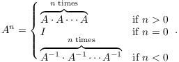
Note that ![]() for
for ![]() only makes sense if A is invertible.
only makes sense if A is invertible.
The usual rules for powers hold:
(a) ![]() .
.
(b) ![]() .
.
The proofs involve induction and taking cases. I don't think they're that enlightening, so I will skip them.
Example. Consider the real matrix
![]()
Compute ![]() and
and ![]() .
.
![]()
Using the formula for the inverse of a ![]() matrix,
matrix,
![]()
Therefore,
![]()
Remember that matrix multiplication isn't commutative, so ![]() is not necessarily equal to
is not necessarily equal to ![]() . So what is
. So what is ![]() ? Since
? Since ![]() is shorthand for
is shorthand for ![]() , and in this case
, and in this case ![]() , the best we can say is that
, the best we can say is that
![]()
Example. Give a specific example of two ![]() real matrices A and B for which
real matrices A and B for which
![]()
How should I construct this counterexample? On the one hand, I want
to avoid matrices which are "too special", because I might
accidentally get a case where the equation holds. (The example in
this problem just shows that the equation "![]() " isn't
always true; this doesn't mean that it's never
true.) For instance, I should not take A to be the identity matrix or
the zero matrix (in which case the equation would actually be true).
" isn't
always true; this doesn't mean that it's never
true.) For instance, I should not take A to be the identity matrix or
the zero matrix (in which case the equation would actually be true).
On the other hand, I'd like to keep the matrices simple --- first, so that I don't struggle to do the computation, and second, so that a reader can easily see that the computation works. For instance, this would be a bad idea:
![$$A = \left[\matrix{-1.378 & \pi \cr \noalign{\vskip2pt} \dfrac{\sqrt{2}}{171} & 1013 \cr}\right].$$](inverses-and-elementary-matrices89.png)
When you're trying to construct a counterexample, try to keep these ideas in mind. In the end, you may have to make a few trials to get a suitable counterexample --- you will not know whether something works without trying.
I will take
![]()
Following the ideas above, I tried to make matrices which were simple without being too special.
Then
![]()
On the other hand,
![]()
So for these two matrices, ![]() .
.![]()
Proposition.
(a) If A and B are invertible ![]() matrices, then
matrices, then ![]() is invertible, and its inverse is given by
is invertible, and its inverse is given by
![]()
(b) If A is invertible, then ![]() is invertible, and its inverse is given by
is invertible, and its inverse is given by
![]()
Proof. (a) Remember that ![]() is not necessarily equal to
is not necessarily equal to ![]() , since matrix multiplication is not
necessarily commutative.
, since matrix multiplication is not
necessarily commutative.
I have
![]()
![]()
Since ![]() gives the identity when
multiplied by
gives the identity when
multiplied by ![]() , it means that
, it means that ![]() must be the inverse of
must be the inverse of ![]() --- that is,
--- that is, ![]() .
.
(b) I have
![]()
Since ![]() gives the
identity when multiplied by
gives the
identity when multiplied by ![]() , it means that
, it means that ![]() must be the inverse of
must be the inverse of ![]() --- that is,
--- that is, ![]() .
.![]()
Remark. Look over the proofs of the two parts of the last proposition and be sure you understand why the computations proved the things that were to be proved. The idea is that the inverse of a matrix is defined by a property, not by appearance. By analogy, it is like the difference between the set of mathematicians (a set defined by a property) and the set of people with purple hair (a set defined by appearance).
A matrix C is the inverse of a matrix D if it has the
property that multiplying C by D (in both orders) gives the
identity I. So to check whether a matrix C really is the
inverse of D, you multiply C by D (in both orders) any see whether
you get I.![]()
Example. Suppose that A and B are ![]() invertible matrices. Simplify the
following expression:
invertible matrices. Simplify the
following expression:
![]()
Note: ![]() is not
is not ![]() , nor is it
, nor is it ![]() .
.
![$$\eqalign{ (A B)^{-2} A (B A)^2 A & = [(A B)^2]^{-1} A (B A)^2 A \cr & = (A B A B)^{-1} A (B A B A) A \cr & = B^{-1} A^{-1} B^{-1} A^{-1} A B A B A A \cr & = A^2 \cr} \quad\halmos$$](inverses-and-elementary-matrices119.png)
Example. ( Solving a matrix equation) Solve the following matrix equation for X, assuming that A and B are invertible:
![]()

Notice that I can multiply both sides of a matrix equation by the
same thing, but I must multiply on the same side of both
sides. So when I multiplied by ![]() , I had to put
, I had to put ![]() on the left side of both sides of
the equation.
on the left side of both sides of
the equation.
Once again, the reason I have to be careful is that in general, ![]() --- matrix multiplication is not
commutative.
--- matrix multiplication is not
commutative.![]()
Example. Give a specific example of two
invertible ![]() real matrices A and B
for which
real matrices A and B
for which
![]()
One way to get a counterexample is to choose A and B so that ![]() isn't invertible. For instance,
isn't invertible. For instance,
![]()
Then A and B happen to be equal to their inverses:
![]()
But
![]()
The zero matrix is not invertible, because ![]() for any matrix C --- so for no
matrix C can
for any matrix C --- so for no
matrix C can ![]() .
.
But this feels like "cheating", because the left side ![]() of the equation isn't defined.
Okay --- can we find two matrices A and B for which
of the equation isn't defined.
Okay --- can we find two matrices A and B for which ![]() and
both sides of the equation are defined? Thus, we need A, B, and
and
both sides of the equation are defined? Thus, we need A, B, and ![]() to all be invertible.
to all be invertible.
I'll use
![]()
Then
![]()
(You can find the inverses using the formula for the inverse of a
![]() matrix which I gave when I
discussed matrix arithmetic. You can also find the inverses using row
reduction.)
matrix which I gave when I
discussed matrix arithmetic. You can also find the inverses using row
reduction.)
Thus,
![]()
On the other hand,
![]()
Thus, ![]() even though both sides of the equation are defined.
even though both sides of the equation are defined.![]()
The next result connects several of the ideas we've looked at: Row reduction, elementary matrices, invertibility, and solving systems of equations.
Theorem. Let A be an ![]() matrix. The following are
equivalent:
matrix. The following are
equivalent:
(a) A is row equivalent to I.
(b) A is a product of elementary matrices.
(c) A is invertible.
(d) The only solution to the following system is the vector ![]() :
:
![]()
(e) For any n-dimensional vector b, the following system has a unique solution:
![]()
Proof. When you are trying to prove several statements are equivalent, you must prove that if you assume any one of the statements, you can prove any of the others. I can do this here by proving that (a) implies (b), (b) implies (c), (c) implies (d), (d) implies (e), and (e) implies (a).
(a) ![]() (b): Let
(b): Let ![]() be elementary matrices which
row reduce A to I:
be elementary matrices which
row reduce A to I:
![]()
Then
![]()
Since the inverse of an elementary matrix is an elementary matrix, A is a product of elementary matrices.
(b) ![]() (c): Write A as
a product of elementary matrices:
(c): Write A as
a product of elementary matrices:
![]()
Now
![]()
![]()
Hence,
![]()
(c) ![]() (d): Suppose A
is invertible. The system
(d): Suppose A
is invertible. The system ![]() has at least one solution, namely
has at least one solution, namely ![]() .
.
Moreover, if y is any other solution, then
![]()
That is, 0 is the one and only solution to the system.
(d) ![]() (e): Suppose
the only solution to
(e): Suppose
the only solution to ![]() is
is ![]() . If
. If ![]() , this means that row reducing the
augmented matrix
, this means that row reducing the
augmented matrix
![$$\left[\matrix{a_{11} & a_{12} & \cdots & a_{1n} & 0 \cr a_{21} & a_{22} & \cdots & a_{2n} & 0 \cr \vdots & \vdots & \ddots & \vdots \cr a_{n1} & a_{n2} & \cdots & a_{nn} & 0 \cr}\right] \quad\hbox{produces}\quad \left[\matrix{1 & 0 & \cdots & 0 & 0 \cr 0 & 1 & \cdots & 0 & 0 \cr \vdots & \vdots & \ddots & \vdots & \vdots \cr 0 & 0 & \cdots & 1 & 0 \cr}\right].$$](inverses-and-elementary-matrices163.png)
Ignoring the last column (which never changes), this means there is a
sequence of row operations ![]() , ...,
, ..., ![]() which reduces A to the identity I --- that
is, A is row equivalent to I. (I've actually proved (d)
which reduces A to the identity I --- that
is, A is row equivalent to I. (I've actually proved (d) ![]() (a) at this point.)
(a) at this point.)
Let ![]() be an arbitrary n-dimensional vector. Then
be an arbitrary n-dimensional vector. Then
![$$E_1\cdots E_n \left[\matrix{a_{11} & a_{12} & \cdots & a_{1n} & b_1 \cr a_{21} & a_{22} & \cdots & a_{2n} & b_2 \cr \vdots & \vdots & \ddots & \vdots \cr a_{n1} & a_{n2} & \cdots & a_{nn} & b_n \cr}\right] = \left[\matrix{1 & 0 & \cdots & 0 & b_1' \cr 0 & 1 & \cdots & 0 & b_2' \cr \vdots & \vdots & \ddots & \vdots & \vdots \cr 0 & 0 & \cdots & 1 & b_n' \cr}\right].$$](inverses-and-elementary-matrices168.png)
Thus, ![]() is a solution.
is a solution.
Suppose y is another solution to ![]() . Then
. Then
![]()
Therefore, ![]() is a solution to
is a solution to ![]() . But the only solution to
. But the only solution to ![]() is 0, so
is 0, so ![]() , or
, or ![]() . Thus,
. Thus, ![]() is the
unique solution to
is the
unique solution to ![]() .
.
(e) ![]() (a): Suppose
(a): Suppose
![]() has a unique solution for every b.
As a special case,
has a unique solution for every b.
As a special case, ![]() has a unique
solution (namely
has a unique
solution (namely ![]() ). But arguing as I
did in (d)
). But arguing as I
did in (d) ![]() (e), I can show
that A row reduces to I, and that is (a).
(e), I can show
that A row reduces to I, and that is (a).![]()
Remark. We'll see that there are many other conditions that are equivalent to a matrix being invertible. For instance, when we study determinants, we'll find that a matrix is invertible if and only if its determinant is invertible as a number.
If A is invertible, the theorem implies that A can be written as a product of elementary matrices. To do this, row reduce A to the identity, keeping track of the row operations you're using. Write each row operation as an elementary matrix, and express the row reduction as a matrix multiplication. Finally, solve the resulting equation for A.
Example. ( Writing an invertible matrix as a product of elementary matrices) Express the following real matrix as a product of elementary matrices:
![]()
First, row reduce A to I:
![]()
![]()
Next, represent each row operation as an elementary matrix:
![$$r_1 \to \dfrac{1}{2}r_1 \quad\hbox{corresponds to}\quad \left[\matrix{\dfrac{1}{2} & 0 \cr \noalign{\vskip2pt} 0 & 1 \cr}\right],$$](inverses-and-elementary-matrices187.png)
![]()
![]()
Using the elementary matrices, write the row reduction as a matrix multiplication. A must be multiplied on the left by the elementary matrices in the order in which the operations were performed.
![$$\left[\matrix{1 & 2 \cr 0 & 1 \cr}\right] \left[\matrix{1 & 0 \cr 2 & 1 \cr}\right] \left[\matrix{\dfrac{1}{2} & 0 \cr \noalign{\vskip2pt} 0 & 1 \cr}\right]\cdot A = I.$$](inverses-and-elementary-matrices190.png)
Solve the last equation for A, being careful to get the inverses in the right order:
![$$\left[\matrix{ \dfrac{1}{2} & 0 \cr \noalign{\vskip2pt} 0 & 1 \cr}\right]^{-1} \left[\matrix{1 & 0 \cr 2 & 1 \cr}\right]^{-1} \left[\matrix{1 & 2 \cr 0 & 1 \cr}\right]^{-1} \left[\matrix{1 & 2 \cr 0 & 1 \cr}\right] \left[\matrix{1 & 0 \cr 2 & 1 \cr}\right] \left[\matrix{\dfrac{1}{2} & 0 \cr \noalign{\vskip2pt} 0 & 1 \cr}\right]\cdot A = \left[\matrix{\dfrac{1}{2} & 0 \cr \noalign{\vskip2pt} 0 & 1 \cr}\right]^{-1} \left[\matrix{1 & 0 \cr 2 & 1 \cr}\right]^{-1} \left[\matrix{1 & 2 \cr 0 & 1 \cr}\right]^{-1}\cdot I,$$](inverses-and-elementary-matrices191.png)
![$$A = \left[\matrix{ \dfrac{1}{2} & 0 \cr \noalign{\vskip2pt} 0 & 1 \cr}\right]^{-1} \left[\matrix{1 & 0 \cr 2 & 1 \cr}\right]^{-1} \left[\matrix{1 & 2 \cr 0 & 1 \cr}\right]^{-1}.$$](inverses-and-elementary-matrices192.png)
Finally, write each inverse as an elementary matrix.
![]()
You can check your answer by multiplying the matrices on the
right.![]()
For two ![]() matrices A and B to be
inverses, I must have
matrices A and B to be
inverses, I must have
![]()
Since in general ![]() need not equal
need not equal ![]() , it seems as though I must check that
both equations hold in order to show that A and B are
inverses. It turns out that, thanks to the earlier theorem, we only
need to check that
, it seems as though I must check that
both equations hold in order to show that A and B are
inverses. It turns out that, thanks to the earlier theorem, we only
need to check that ![]() .
.
Corollary. If A and B are ![]() matrices and
matrices and ![]() , then
, then ![]() and
and ![]() .
.
Proof. Suppose A and B are ![]() matrices and
matrices and ![]() . The system
. The system ![]() certainly has
certainly has ![]() as a solution. I'll show it's the only
solution.
as a solution. I'll show it's the only
solution.
Suppose y is another solution, so
![]()
Multiply both sides by A and simplify:

Thus, 0 is a solution, and it's the only solution.
Thus, B satisfies condition (d) of the Theorem. Since the five
conditions are equivalent, B also satisfies condition (c), so B is
invertible. Let ![]() be the inverse of
B. Then
be the inverse of
B. Then
This proves the first part of the Corollary. Finally,
![]()
This finishes the proof.![]()
The proof of the theorem gives an algorithm for inverting a matrix A.
If A is invertible, there are elementary matrices ![]() which row reduce A to I:
which row reduce A to I:
![]()
But this equation says that ![]() is the inverse of A, since
multiplying A by
is the inverse of A, since
multiplying A by ![]() gives the
identity. Thus,
gives the
identity. Thus,
![]()
We can interpret the last expression ![]() as applying the row
operations for
as applying the row
operations for ![]() , ...
, ... ![]() to the identity matrix I. And the same row
operations row reduce A to I. So form an augmented matrix by placing
the identity matrix next to A:
to the identity matrix I. And the same row
operations row reduce A to I. So form an augmented matrix by placing
the identity matrix next to A:
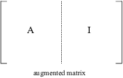
Row reduce the augmented matrix. The left-hand block A will row
reduce to the identity; at the same time, the right-hand block I will
be transformed into ![]() .
.
Example. Invert the following matrix over ![]() :
:
![$$\left[\matrix{ 1 & 2 & -1 \cr -1 & -1 & 3 \cr 0 & 1 & 1 \cr}\right].$$](inverses-and-elementary-matrices223.png)
Form the augmented matrix by putting the ![]() identity matrix on the right of
the original matrix:
identity matrix on the right of
the original matrix:
![$$\left[\matrix{ 1 & 2 & -1 \cr -1 & -1 & 3 \cr 0 & 1 & 1 \cr}\right| \left.\matrix{ 1 & 0 & 0 \cr 0 & 1 & 0 \cr 0 & 0 & 1 \cr}\right].$$](inverses-and-elementary-matrices225.png)
Next, row reduce the augmented matrix. The row operations are entirely determined by the block on the left, which is the original matrix. The row operations turn the left block into the identity, while simultaneously turning the identity in the right block into the inverse.
![$$\left[\matrix{ 1 & 2 & -1 \cr -1 & -1 & 3 \cr 0 & 1 & 1 \cr}\right| \left.\matrix{ 1 & 0 & 0 \cr 0 & 1 & 0 \cr 0 & 0 & 1 \cr}\right] \quad\matrix{\rightarrow \cr r_2 \to r_2 + r_1 \cr}\quad \left[\matrix{ 1 & 2 & -1 \cr 0 & 1 & 2 \cr 0 & 1 & 1 \cr}\right| \left.\matrix{ 1 & 0 & 0 \cr 1 & 1 & 0 \cr 0 & 0 & 1 \cr}\right] \quad\matrix{\rightarrow \cr r_3 \to r_3 - r_2 \cr}$$](inverses-and-elementary-matrices226.png)
![$$\left[\matrix{ 1 & 2 & -1 \cr 0 & 1 & 2 \cr 0 & 0 & -1 \cr}\right| \left.\matrix{ 1 & 0 & 0 \cr 1 & 1 & 0 \cr -1 & -1 & 1 \cr}\right] \quad\matrix{\rightarrow \cr r_1 \to r_1 - 2 r_2 \cr}\quad \left[\matrix{ 1 & 0 & -5 \cr 0 & 1 & 2 \cr 0 & 0 & -1 \cr}\right| \left.\matrix{ -1 & -2 & 0 \cr 1 & 1 & 0 \cr -1 & -1 & 1 \cr}\right] \quad\matrix{\rightarrow \cr r_3 \to -r_3 \cr}$$](inverses-and-elementary-matrices227.png)
![$$\left[\matrix{ 1 & 0 & -5 \cr 0 & 1 & 2 \cr 0 & 0 & 1 \cr}\right| \left.\matrix{ -1 & -2 & 0 \cr 1 & 1 & 0 \cr 1 & 1 & -1 \cr}\right] \quad\matrix{\rightarrow \cr r_1 \to r_1 + 5 r_3 \cr}\quad \left[\matrix{ 1 & 0 & 0 \cr 0 & 1 & 2 \cr 0 & 0 & 1 \cr}\right| \left.\matrix{ 4 & 3 & -5 \cr 1 & 1 & 0 \cr 1 & 1 & -1 \cr}\right] \quad\matrix{\rightarrow \cr r_2 \to r_2 - 2 r_3 \cr}$$](inverses-and-elementary-matrices228.png)
![$$\left[\matrix{ 1 & 0 & 0 \cr 0 & 1 & 0 \cr 0 & 0 & 1 \cr}\right| \left.\matrix{ 4 & 3 & -5 \cr -1 & -1 & 2 \cr 1 & 1 & -1 \cr}\right].$$](inverses-and-elementary-matrices229.png)
Thus,
![$$\left[\matrix{ 1 & 2 & -1 \cr -1 & -1 & 3 \cr 0 & 1 & 1 \cr}\right]^{-1} = \left[\matrix{ 4 & 3 & -5 \cr -1 & -1 & 2 \cr 1 & 1 & -1 \cr}\right].\quad\halmos$$](inverses-and-elementary-matrices230.png)
In the future, I won't draw the vertical bar between the two blocks; you can draw it if it helps you keep the computation organized.
Example. ( Inverting a matrix
over ![]() ) Find the
inverse of the following matrix over
) Find the
inverse of the following matrix over ![]() :
:
![$$\left[\matrix{ 1 & 0 & 2 \cr 1 & 1 & 1 \cr 2 & 1 & 1 \cr}\right].$$](inverses-and-elementary-matrices233.png)
Form the augmented matrix and row reduce:
![$$\left[\matrix{ 1 & 0 & 2 & 1 & 0 & 0 \cr 1 & 1 & 1 & 0 & 1 & 0 \cr 2 & 1 & 1 & 0 & 0 & 1 \cr}\right] \matrix{\rightarrow \cr r_2 \to r_2 - r_1 \cr} \left[\matrix{ 1 & 0 & 2 & 1 & 0 & 0 \cr 0 & 1 & 2 & 2 & 1 & 0 \cr 2 & 1 & 1 & 0 & 0 & 1 \cr}\right] \matrix{\rightarrow \cr r_3 \to r_3 - 2 r_1 \cr}$$](inverses-and-elementary-matrices234.png)
![$$\left[\matrix{ 1 & 0 & 2 & 1 & 0 & 0 \cr 0 & 1 & 2 & 2 & 1 & 0 \cr 0 & 1 & 0 & 1 & 0 & 1 \cr}\right] \matrix{\rightarrow \cr r_3 \to r_3 - r_2 \cr} \left[\matrix{ 1 & 0 & 2 & 1 & 0 & 0 \cr 0 & 1 & 2 & 2 & 1 & 0 \cr 0 & 0 & 1 & 2 & 2 & 1 \cr}\right] \matrix{\rightarrow \cr r_1 \to r_1 - 2 r_3 \cr}$$](inverses-and-elementary-matrices235.png)
![$$\left[\matrix{ 1 & 0 & 0 & 0 & 2 & 1 \cr 0 & 1 & 2 & 2 & 1 & 0 \cr 0 & 0 & 1 & 2 & 2 & 1 \cr}\right] \matrix{\rightarrow \cr r_2 \to r_2 - 2 r_3 \cr} \left[\matrix{ 1 & 0 & 0 & 0 & 2 & 1 \cr 0 & 1 & 0 & 1 & 0 & 1 \cr 0 & 0 & 1 & 2 & 2 & 1 \cr}\right]$$](inverses-and-elementary-matrices236.png)
Therefore,
![$$\left[\matrix{ 1 & 0 & 2 \cr 1 & 1 & 1 \cr 2 & 1 & 1 \cr}\right]^{-1} = \left[\matrix{ 0 & 2 & 1 \cr 1 & 0 & 1 \cr 2 & 2 & 1 \cr}\right].\quad\halmos$$](inverses-and-elementary-matrices237.png)
The theorem also tells us about the number of solutions to a system of linear equations.
Proposition. Let F be a field, and let ![]() be a system of linear equations
over F. Then:
be a system of linear equations
over F. Then:
(a) If F is infinite, then the system has either no solutions, exactly one solution, or infinitely many solutions.
(b) If F is a finite field with ![]() elements, where p is prime and
elements, where p is prime and ![]() , then the system has either no
solutions, exactly one solution, or at least
, then the system has either no
solutions, exactly one solution, or at least ![]() solutions.
solutions.
Proof. Suppose the system has more than one
solution. I must show that there are infinitely many solutions if F
is infinite, or at least ![]() solutions if F is a finite field with
solutions if F is a finite field with ![]() elements.
elements.
Since there is more than one solution, there are at least two
different solutions. So let ![]() and
and ![]() be two different solutions to
be two different solutions to ![]() :
:
![]()
Subtracting the equations gives
![]()
Since ![]() ,
, ![]() is a nontrivial solution to the
system
is a nontrivial solution to the
system ![]() . Now if
. Now if ![]() ,
,
![]()
Thus, ![]() is a solution to
is a solution to
![]() . Moreover, the only way two
solutions of the form
. Moreover, the only way two
solutions of the form ![]() can be the same is if they
have the same t. For
can be the same is if they
have the same t. For
![]()
Since ![]() , I have
, I have ![]() . So I can divide both sides by
. So I can divide both sides by
![]() , and I get
, and I get ![]() .
.
Thus, different t's give different ![]() 's, each of which is a
solution to the system.
's, each of which is a
solution to the system.
If F has infinitely many elements, there are infinitely many possibilities for t, so there are infinitely many solutions.
If F has ![]() elements, there are
elements, there are
![]() possibilities for t, so there are
at least
possibilities for t, so there are
at least ![]() solutions. (Note that
there may be solutions which are not of the form
solutions. (Note that
there may be solutions which are not of the form ![]() , so there may be more
than
, so there may be more
than ![]() solutions. In fact, I'll be able
to show later than the number of solutions will be some power of
solutions. In fact, I'll be able
to show later than the number of solutions will be some power of ![]() .)
.)![]()
For example, since ![]() is an infinite
field, a system of linear equations over
is an infinite
field, a system of linear equations over ![]() has no solutions, exactly one solution, or
infinitely many solutions.
has no solutions, exactly one solution, or
infinitely many solutions.
On the other hand, since ![]() is a field with 3 elements, a
system of linear equations over
is a field with 3 elements, a
system of linear equations over ![]() has no solutions, exactly one
solution, or at least 3 solutions. (And I'll see later that if
there's more than one solution, then there might be 3 solutions, 9
solutions, 27 solutions, ....)
has no solutions, exactly one
solution, or at least 3 solutions. (And I'll see later that if
there's more than one solution, then there might be 3 solutions, 9
solutions, 27 solutions, ....)
Copyright 2021 by Bruce Ikenaga