In this section, all of the matrices will be real or complex matrices.
The solution to the exponential growth equation
![]()
A constant coefficient linear system has a similar form, but we have vectors and a matrix instead of scalars:
![]()
Thus, if A is an ![]() real matrix, then
real matrix, then ![]() .
.
It's natural to ask whether you can solve a constant coefficient linear system using some kind of exponential, as with the exponential growth equation.
If a solution to the system is to have the same form as the growth equation solution, it should look like
![]()
But "![]() " seems to be e raised to a matrix
power! How does that make any sense? It turns out that the matrix exponential
" seems to be e raised to a matrix
power! How does that make any sense? It turns out that the matrix exponential ![]() can be defined in a reasonable way.
can be defined in a reasonable way.
From calculus, the Taylor series for ![]() is
is
![]()
It converges absolutely for all z.
It A is an ![]() matrix with real entries, define
matrix with real entries, define
![]()
The powers ![]() make sense, since A is a square matrix. It
is possible to show that this series converges for all t and every
matrix A.
make sense, since A is a square matrix. It
is possible to show that this series converges for all t and every
matrix A.
As a consequence, I can differentiate the series term-by-term:
![]()
This shows that ![]() solves the differential equation
solves the differential equation
![]() . The initial condition vector
. The initial condition vector ![]() yields the particular solution
yields the particular solution
![]()
This works, because ![]() (by setting
(by setting ![]() in the power series).
in the power series).
Another familiar property of ordinary exponentials holds for the
matrix exponential: If A and B commute (that is, ![]() ), then
), then
![]()
You can prove this by multiplying the power series for the
exponentials on the left. (![]() is just
is just ![]() with
with ![]() .)
.)
Example. Compute ![]() if
if
![]()
Compute the successive powers of A:
![]()
Therefore,
![$$e^{A t} = \sum_{n = 0}^\infty \dfrac{t^n}{n!} \left[\matrix{2^n & 0 \cr 0 & 3^n \cr}\right] = \left[\matrix{\sum_{n = 0}^\infty \dfrac{(2 t)^n}{n!} & 0 \cr \noalign{\vskip2 pt} 0 & \sum_{n = 0}^\infty \dfrac{(3 t)^n}{n!} \cr}\right] = \left[\matrix{e^{2 t} & 0 \cr 0 & e^{3 t} \cr}\right].\quad\halmos$$](matrix-exponential28.png)
You can compute the exponential of an arbitrary diagonal matrix in the same way:
![$$A = \left[\matrix{\lambda_1 & 0 & \cdots & 0 \cr 0 & \lambda_2 & \cdots & 0 \cr \vdots & \vdots & & \vdots \cr 0 & 0 & \cdots & \lambda_n \cr}\right], \quad e^{A t} = \left[\matrix{e^{\lambda_1 t} & 0 & \cdots & 0 \cr 0 & e^{\lambda_2 t} & \cdots & 0 \cr \vdots & \vdots & & \vdots \cr 0 & 0 & \cdots & e^{\lambda_n t} \cr}\right].$$](matrix-exponential29.png)
For example, if
![$$A = \left[\matrix{ -3 & 0 & 0 \cr 0 & 4 & 0 \cr 0 & 0 & 1.73 \cr}\right], \quad\hbox{then}\quad e^{A t} = \left[\matrix{ e^{-3 t} & 0 & 0 \cr 0 & e^{4 t} & 0 \cr 0 & 0 & e^{1.73 t} \cr}\right].$$](matrix-exponential30.png)
Using this idea, we can compute ![]() when A is
diagonalizable. First, I'll give examples where we can compute
when A is
diagonalizable. First, I'll give examples where we can compute ![]() : First, using a "lucky" pattern, and
second, using our knowledge of how to solve a system of differential
equations.
: First, using a "lucky" pattern, and
second, using our knowledge of how to solve a system of differential
equations.
Example. Compute ![]() if
if
![]()
Compute the successive powers of A:
![]()
Hence,
![$$e^{A t} = \sum_{n = 0}^\infty \dfrac{t^n}{n!} \left[\matrix{1 & 2 n \cr 0 & 1 \cr}\right] = \left[\matrix{\sum_{n = 0}^\infty \dfrac{t^n}{n!} & \sum_{n = 0}^\infty \dfrac{2 n t^n}{n!} \cr \noalign{\vskip2 pt} 0 & \sum_{n = 0}^\infty \dfrac{t^n}{n!} \cr}\right] = \left[\matrix{e^t & 2 t e^t \cr 0 & e^t \cr}\right].$$](matrix-exponential36.png)
Here's where the last equality came from:
![]()
![]()
In the last example, we got lucky in being able to recognize a pattern in the terms of the power series. Here is what happens if we aren't so lucky.
Example. Compute ![]() , if
, if
![]()
If you compute powers of A as in the last two examples, there is no evident pattern:
![]()
It looks like it would be difficult to compute the matrix exponential using the power series.
I'll use the fact that ![]() is the solution to a linear
system. The system's coefficient matrix is A, so the system is
is the solution to a linear
system. The system's coefficient matrix is A, so the system is
![]()
You can solve this system by hand. For instance, the first equation gives
![]()
Plugging these expressions for y and ![]() into
into ![]() , I get
, I get
![]()
After some simplification, this becomes
![]()
The solution is
![]()
Plugging this into the expression for y above and doing some ugly algebra gives
![]()
Next, remember that if B is a ![]() matrix,
matrix,
![]()
Try this out with a particular B to see how it works.
In particular, this is true for ![]() . Now
. Now ![]() is the solution satisfying
is the solution satisfying ![]() , but
, but
![$$x = \left[\matrix{ c_1 e^t + c_2 e^{-2 t} \cr \noalign{\vskip2 pt} \dfrac{1}{5} c_1 e^t + \dfrac{1}{2} c_2 e^{-2 t} \cr}\right].$$](matrix-exponential56.png)
Set ![]() to get the first column of
to get the first column of ![]() :
:
![$$\left[\matrix{1 \cr 0 \cr}\right] = \left[\matrix{ c_1 + c_2 \cr \noalign{\vskip2 pt} \dfrac{1}{5} c_1 + \dfrac{1}{2} c_2 \cr}\right].$$](matrix-exponential59.png)
Solving this system of equations for ![]() and
and ![]() , I get
, I get ![]() ,
, ![]() . So
. So
![$$\left[\matrix{x \cr y \cr}\right] = \left[\matrix{ \dfrac{5}{3} e^t - \dfrac{2}{3} e^{-2 t} \cr \noalign{\vskip2 pt} \dfrac{1}{3} e^t - \dfrac{1}{3} e^{-2 t} \cr}\right].$$](matrix-exponential64.png)
Set ![]() to get the second column of
to get the second column of ![]() :
:
![$$\left[\matrix{0 \cr 1 \cr}\right] = \left[\matrix{ c_1 + c_2 \cr \noalign{\vskip2 pt} \dfrac{1}{5} c_1 + \dfrac{1}{2} c_2 \cr}\right].$$](matrix-exponential67.png)
Therefore, ![]() ,
, ![]() . Hence,
. Hence,
![$$\left[\matrix{x \cr y \cr}\right] = \left[\matrix{ -\dfrac{10}{3} e^t + \dfrac{10}{3} e^{-2 t} \cr \noalign{\vskip2 pt} -\dfrac{2}{3} e^t + \dfrac{5}{3} e^{-2 t} \cr}\right].$$](matrix-exponential70.png)
Therefore,
![$$e^{A t} = \left[\matrix{ \dfrac{5}{3} e^t - \dfrac{2}{3} e^{-2 t} & -\dfrac{10}{3} e^t + \dfrac{10}{3} e^{-2 t} \cr \noalign{\vskip2 pt} \dfrac{1}{3} e^t - \dfrac{1}{3} e^{-2 t} & -\dfrac{2}{3} e^t + \dfrac{5}{3} e^{-2 t} \cr}\right].$$](matrix-exponential71.png)
So I found ![]() , but this was a lot of work (not
all of which I wrote out!), and A was just a
, but this was a lot of work (not
all of which I wrote out!), and A was just a ![]() matrix.
matrix.![]()
We noted earlier that we can compute ![]() fairly easily in case A is diagonalizable. Recall
that an
fairly easily in case A is diagonalizable. Recall
that an ![]() matrix A is
diagonalizable if it has n independent eigenvectors. (This is
true, for example, if A has n distinct eigenvalues.)
matrix A is
diagonalizable if it has n independent eigenvectors. (This is
true, for example, if A has n distinct eigenvalues.)
Suppose A is diagonalizable with independent eigenvectors ![]() and corresponding eigenvalues
and corresponding eigenvalues ![]() . Let S be the matrix whose
columns are the eigenvectors:
. Let S be the matrix whose
columns are the eigenvectors:
![$$S = \left[\matrix{ \uparrow & \uparrow & & \uparrow \cr v_1 & v_2 & \cdots & v_n \cr \downarrow & \downarrow & & \downarrow \cr}\right].$$](matrix-exponential78.png)
Then
![$$S^{-1} A S = \left[\matrix{ \lambda_1 & 0 & \cdots & 0 \cr 0 & \lambda_2 & \cdots & 0 \cr \vdots & \vdots & & \vdots \cr 0 & 0 & \cdots & \lambda_n \cr}\right] = D.$$](matrix-exponential79.png)
We saw earlier how to compute the exponential for the diagonal matrix D:
![$$e^{D t} = \left[\matrix{ e^{\lambda_1 t} & 0 & \cdots & 0 \cr 0 & e^{\lambda_2 t} & \cdots & 0 \cr \vdots & \vdots & & \vdots \cr 0 & 0 & \cdots & e^{\lambda_n t} \cr}\right].$$](matrix-exponential80.png)
But note that
![]()
Notice how each "![]() " pair cancels.
Continuing in this way --- you can give a formal proof using
induction --- we have
" pair cancels.
Continuing in this way --- you can give a formal proof using
induction --- we have ![]() . Therefore,
. Therefore,
![]()
Then
![]()
Notice that S and ![]() have "switched places"
from the original diagonalization equation.
have "switched places"
from the original diagonalization equation.
Hence,
![$$e^{A t} = S \left[\matrix{ e^{\lambda_1 t} & 0 & \cdots & 0 \cr 0 & e^{\lambda_2 t} & \cdots & 0 \cr \vdots & \vdots & & \vdots \cr 0 & 0 & \cdots & e^{\lambda_n t} \cr}\right] S^{-1}.$$](matrix-exponential87.png)
Thus, if A is diagonalizable, find the eigenvalues and use them to
construct the diagonal matrix with the exponentials in the middle.
Find a set of independent eigenvectors and use them to construct S
and ![]() . Putting everything into the equation
above gives
. Putting everything into the equation
above gives ![]() .
.
Example. Compute ![]() if
if
![]()
The characteristic polynomial is ![]() and the
eigenvalues are
and the
eigenvalues are ![]() ,
, ![]() . Since there are two different eigenvalues
and A is a
. Since there are two different eigenvalues
and A is a ![]() matrix, A is diagonalizable. The
corresponding eigenvectors are
matrix, A is diagonalizable. The
corresponding eigenvectors are ![]() and
and ![]() . Thus,
. Thus,
![]()
Hence,
![]()
Example. Compute ![]() if
if
![$$A = \left[\matrix{ 5 & -6 & -6 \cr -1 & 4 & 2 \cr 3 & -6 & -4 \cr}\right].$$](matrix-exponential101.png)
The characteristic polynomial is ![]() and the
eigenvalues are
and the
eigenvalues are ![]() and
and ![]() (a double root). The corresponding
eigenvectors are
(a double root). The corresponding
eigenvectors are ![]() for
for ![]() , and
, and ![]() and
and ![]() for
for ![]() . Since I have
3 independent eigenvectors, the matrix is diagonalizable.
. Since I have
3 independent eigenvectors, the matrix is diagonalizable.
I have
![$$S = \left[\matrix{ 3 & 2 & 2 \cr -1 & 1 & 0 \cr 3 & 0 & 1 \cr}\right], \quad S^{-1} = \left[\matrix{ -1 & 2 & 2 \cr -1 & 3 & 2 \cr 3 & -6 & -5 \cr}\right].$$](matrix-exponential110.png)
From this, it follows that
![$$e^{A t} = \left[\matrix{ -3 e^t + 4 e^{2 t} & 6 e^t - 6 e^{2 t} & 6 e^t - 6 e^{2 t} \cr e^t - e^{2 t} & -2 e^t + 3 e^{2 t} & -2 e^t + 2 e^{2 t} \cr -3 e^t + 3 e^{2 t} & 6 e^t - 6 e^{2 t} & 6 e^t - 5 e^{2 t} \cr}\right].\quad\halmos$$](matrix-exponential111.png)
Here's a quick check you can use when computing ![]() . Plugging
. Plugging ![]() into
into ![]() gives
gives ![]() , the identity matrix. For
instance, in the last example, if you set
, the identity matrix. For
instance, in the last example, if you set ![]() in the right side, it checks:
in the right side, it checks:
![$$\left[\matrix{ 1 & 0 & 0 \cr 0 & 1 & 0 \cr 0 & 0 & 1 \cr}\right].$$](matrix-exponential117.png)
However, this check isn't foolproof --- just because you get I by
setting ![]() doesn't mean your answer is right. However,
if you don't get I, your answer is surely wrong!
doesn't mean your answer is right. However,
if you don't get I, your answer is surely wrong!
A better check that is a little more work is to compute the
derivative of ![]() , and then set
, and then set ![]() . You should get A. To see this, note that
. You should get A. To see this, note that
![]()
Evaluating both sides of this equation at ![]() gives
gives ![]() . Since the theory of differential
equations tells us that the solution to an initial value problem of
this kind is unique, if your answer passes these checks then it
is
. Since the theory of differential
equations tells us that the solution to an initial value problem of
this kind is unique, if your answer passes these checks then it
is ![]() . I think it's good to do the
first (easier) check, even if you don't do the second.
. I think it's good to do the
first (easier) check, even if you don't do the second.
If you try this in the previous example, you'll find that the second check works as well.
Unfortunately, not every matrix is diagonalizable. How do we compute
![]() for an arbitrary real matrix?
for an arbitrary real matrix?
One approach is to use the Jordan canonical form for a matrix, but this would require a discussion of canonical forms, a large subject in itself.
Note that any method for finding ![]() requires finding
the eigenvalues of A which is, in general, a difficult problem. For
instance, there are methods from numerical analysis for
approximating the eigenvalues of a matrix.
requires finding
the eigenvalues of A which is, in general, a difficult problem. For
instance, there are methods from numerical analysis for
approximating the eigenvalues of a matrix.
I'll describe an iterative algorithm for computing ![]() that only requires that one know the eigenvalues of
A. There are various such algorithms for computing the matrix
exponential; this one, which is due to Richard Williamson [1], seems
to me to be the easiest for hand computation. It's also possible to
implement this method using a computer algebra system like
maxima or Mathematica.
that only requires that one know the eigenvalues of
A. There are various such algorithms for computing the matrix
exponential; this one, which is due to Richard Williamson [1], seems
to me to be the easiest for hand computation. It's also possible to
implement this method using a computer algebra system like
maxima or Mathematica.
Let A be an ![]() matrix. Let
matrix. Let ![]() be a list of the
eigenvalues, with multiple eigenvalues repeated according to their
multiplicity.
be a list of the
eigenvalues, with multiple eigenvalues repeated according to their
multiplicity.
The last phrase means that if the characteristic polynomial is ![]() , the eigenvalue 1 is listed 3 times. So
your list of eigenvalues might be
, the eigenvalue 1 is listed 3 times. So
your list of eigenvalues might be ![]() . But you can list them in any order; if
you wanted to show off, you could make your list
. But you can list them in any order; if
you wanted to show off, you could make your list ![]() . It will probably make the computations
easier and less error-prone if you list the eigenvalues in some
"nice" way (so either
. It will probably make the computations
easier and less error-prone if you list the eigenvalues in some
"nice" way (so either ![]() or
or ![]() ).
).
Let
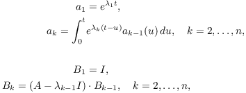
Then
![]()
Remark. If you've seen
convolutions before, you might recognize that the expression for
![]() is a convolution:
is a convolution:
![]()
In general, the convolution of f and g is
![]()
If you haven't seen this before, don't worry: you do not need to know
this! The important thing (which gives the definition of ![]() ) is the integral on the right side.
) is the integral on the right side.
To prove that this algorithm works, I'll show that the expression on
the right satisfies the differential equation ![]() . To do this, I'll need two facts about the
characteristic polynomial
. To do this, I'll need two facts about the
characteristic polynomial ![]() .
.
1. ![]() .
.
2. ( Cayley-Hamilton Theorem) ![]() .
.
Observe that if ![]() is the characteristic polynomial,
then using the first fact and the definition of the B's,
is the characteristic polynomial,
then using the first fact and the definition of the B's,
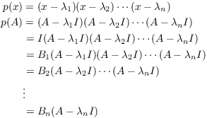
By the Cayley-Hamilton Theorem,
![]()
I will use this fact in the proof below. First, let's see an example of the Cayley-Hamilton theorem. Let
![]()
The characteristic polynomial is ![]() . The Cayley-Hamilton theorem asserts that if you
plug A into
. The Cayley-Hamilton theorem asserts that if you
plug A into ![]() , you'll get the zero matrix.
, you'll get the zero matrix.
First,
![]()
Therefore,
![]()
We've verified the Cayley-Hamilton theorem for this matrix. We'll
provide a proof elsewhere. Let's give a proof of the algorithm for
![]() .
.
Proof of the algorithm. First,
![]()
Recall that the Fundamental Theorem of Calculus says that
![]()
Applying this and the Product Rule, I can differentiate ![]() to obtain
to obtain
![]()
![]()
Therefore,
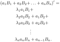
Expand the ![]() terms using
terms using
![]()
Making this substitution and telescoping the sum, I have
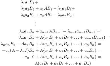
(The result (*) proved above was used in the next-to-the-last equality.) Combining the results above, I've shown that
![]()
This shows that ![]() satisfies
satisfies ![]() .
.
Using the power series expansion, I have ![]() . So
. So
![]()
(Remember that matrix multiplication is not commutative in general!)
It follows that ![]() is a constant matrix.
is a constant matrix.
Set ![]() . Since
. Since ![]() , it follows that
, it follows that ![]() . In addition,
. In addition, ![]() .
Therefore,
.
Therefore, ![]() , and hence
, and hence ![]() .
.![]()
Example. Use the matrix exponential to solve
![]()
![]() is the solution vector.
is the solution vector.
The characteristic polynomial is ![]() . You can check
that there is only one independent eigenvector, so I can't solve the
system by diagonalizing. I could use generalized
eigenvectors to solve the system, but I will use the matrix
exponential to illustrate the algorithm.
. You can check
that there is only one independent eigenvector, so I can't solve the
system by diagonalizing. I could use generalized
eigenvectors to solve the system, but I will use the matrix
exponential to illustrate the algorithm.
First, list the eigenvalues: ![]() . Since
. Since ![]() is a double root, it is listed twice.
is a double root, it is listed twice.
First, I'll compute the ![]() 's:
's:
![]()
![]()
Here are the ![]() 's:
's:
![]()
Therefore,
![]()
As a rough check, note that setting ![]() produces the identity.)
produces the identity.)
The solution to the given initial value problem is
![]()
You can get the general solution by replacing ![]() with
with ![]() .
.![]()
Example. Find ![]() if
if
![$$A = \left[\matrix{ 1 & 0 & 0 \cr 1 & 1 & 0 \cr -1 & -1 & 2 \cr}\right].$$](matrix-exponential191.png)
The eigenvalues are obviously ![]() (double) and
(double) and
![]() .
.
First, I'll compute the ![]() 's. I have
's. I have ![]() , and
, and
![]()
![]()
Next, I'll compute the ![]() 's.
's. ![]() , and
, and
![$$B_2 = A - I = \left[\matrix{ 0 & 0 & 0 \cr 1 & 0 & 0 \cr -1 & -1 & 1 \cr}\right],$$](matrix-exponential200.png)
![$$B_3 = (A - I)B_2 = \left[\matrix{ 0 & 0 & 0 \cr 0 & 0 & 0 \cr -2 & -1 & 1 \cr}\right].$$](matrix-exponential201.png)
Therefore,
![$$e^{A t} = \left[\matrix{ e^t & 0 & 0 \cr t e^t & e^t & 0 \cr t e^t + 2 e^t - 2 e^{2 t} & e^t - e^{2 t} & e^{2 t} \cr}\right].\quad\halmos$$](matrix-exponential202.png)
Example. Use the matrix exponential to solve
![]()
![]() is the solution vector.
is the solution vector.
This example will demonstrate how the algorithm for ![]() works when the eigenvalues are complex.
works when the eigenvalues are complex.
The characteristic polynomial is ![]() . The
eigenvalues are
. The
eigenvalues are ![]() . I will list them as
. I will list them as
![]() .
.
First, I'll compute the ![]() 's.
's. ![]() , and
, and
![]()
![]()
Next, I'll compute the ![]() 's.
's. ![]() , and
, and
![]()
Therefore,
![]()
I want a real solution, so I'll use DeMoivre's Formula to simplify:
Plugging these into the expression for ![]() above, I have
above, I have
![]()
Notice that all the i's have dropped out! This reflects the obvious fact that the exponential of a real matrix must be a real matrix.
Finally, the general solution to the original system is
![]()
Example. Solve the following system using both the matrix exponential and the eigenvector methods.
![]()
![]() is the solution vector.
is the solution vector.
The characteristic polynomial is ![]() . The
eigenvalues are
. The
eigenvalues are ![]() .
.
Consider ![]() :
:
![]()
As this is an eigenvector matrix, it must be singular, and hence the
rows must be multiples. So ignore the second row. I want a vector
![]() such that
such that ![]() . To get such a vector, switch the
. To get such a vector, switch the ![]() and -1 and negate one of them:
and -1 and negate one of them: ![]() ,
, ![]() . Thus,
. Thus, ![]() is an eigenvector.
is an eigenvector.
The corresponding solution is
![]()
Take the real and imaginary parts:
![]()
![]()
The solution is
![]()
Now I'll solve the equation using the matrix exponential. The
eigenvalues are ![]() . Compute the
. Compute the ![]() 's.
's. ![]() , and
, and
![]()
![]()
(Here and below, I'm cheating a little in the comparison by not showing all the algebra involved in the simplification. You need to use DeMoivre's Formula to eliminate the complex exponentials.)
Next, compute the ![]() 's.
's. ![]() , and
, and
![]()
Therefore,
![]()
The solution is
![]()
Taking into account some of the algebra I didn't show for the matrix
exponential, I think the eigenvector approach is easier.![]()
Example. Solve the following system using both the matrix exponential and the (generalized) eigenvector methods.
![]()
![]() is the solution vector.
is the solution vector.
I'll do this first using the generalized eigenvector method, then using the matrix exponential.
The characteristic polynomial is ![]() . The
eigenvalue is
. The
eigenvalue is ![]() (double).
(double).
![]()
Ignore the first row, and divide the second row by 2, obtaining the
vector ![]() . I want
. I want ![]() such that
such that ![]() . Swap 1
and -2 and negate the -2: I get
. Swap 1
and -2 and negate the -2: I get ![]() . This is
an eigenvector for
. This is
an eigenvector for ![]() .
.
Since I only have one eigenvector, I need a generalized eigenvector.
This means I need ![]() such that
such that
![]()
Row reduce:
![$$\left[\matrix{ 4 & -8 & 2 \cr 2 & -4 & 1 \cr}\right] \quad \to \quad \left[\matrix{ 1 & -2 & \dfrac{1}{2} \cr \noalign{\vskip2 pt} 0 & 0 & 0 \cr}\right]$$](matrix-exponential259.png)
This means that ![]() . Setting
. Setting ![]() yields
yields ![]() . The generalized
eigenvector is
. The generalized
eigenvector is ![]() .
.
The solution is
![$$y = c_1 e^t \left[\matrix{2 \cr 1 \cr}\right] + c_2\left(t e^t \left[\matrix{2 \cr 1 \cr}\right] + e^t \left[\matrix{\dfrac{1}{2} \cr \noalign{\vskip2 pt} 0 \cr}\right]\right).$$](matrix-exponential264.png)
Next, I'll solve the system using the matrix exponential. The
eigenvalues are ![]() . First, I'll compute the
. First, I'll compute the ![]() 's.
's. ![]() , and
, and
![]()
Next, compute the ![]() 's.
's. ![]() , and
, and
![]()
Therefore,
![]()
The solution is
![]()
In this case, finding the solution using the matrix exponential may
be a little bit easier.![]()
[1] Richard Williamson, Introduction to differential equations. Englewood Cliffs, NJ: Prentice-Hall, 1986.
Copyright 2023 by Bruce Ikenaga