Systems of linear equations occur frequently in math and in applications. I'll explain what they are, and then how to use row reduction to solve them.
Systems of linear equations
If ![]() ,
, ![]() , ...,
, ..., ![]() , b are numbers and
, b are numbers and ![]() ,
, ![]() , ...,
, ..., ![]() are variables, a linear
equation is an equation of the form
are variables, a linear
equation is an equation of the form
![]()
The a's are referred to as the coefficients and b is the constant term. If the number of variables is small, we may use unsubscripted variables (like x, y, z).
For the moment I won't be specific about what number system we're using; if you want, you can think of some commutative ring with identity. In a particular situation, the number system will be specified.
And as usual, any equation which is algebraically equivalent to the one above is considered a linear equation; for example,
![]()
But I will almost always write linear equations in the first form, with the variable terms on one side and the constant term on the other.
A system of linear equations is a collection of linear equations
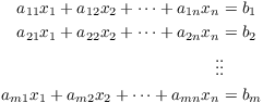
All the a's and b's are assumed to come from some number system.
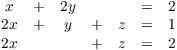
For example, here are some systems of linear equations with
coefficients in ![]() :
:
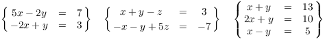
(The curly braces around each system are just here to make them stand out; if there's no chance of confusion, they aren't necessary.)
A solution to a system of linear equations is a set of values for the variables which makes all the equations true. For example,
![]()
You can check this by plugging in:
![]()
Note that we consider the pair ![]() a single solution
to the system. In fact, it's the only solution to this
system of equations.
a single solution
to the system. In fact, it's the only solution to this
system of equations.
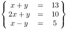
Likewise, you can check that ![]() and
and ![]() are solutions to
are solutions to
![]()
They aren't the only solutions: In fact, this system has an infinite number of solutions.
This system has no solutions:
Here's one way to see this. Add the first and third equations to get
![]() , which means
, which means ![]() . Plug
. Plug ![]() into the second equation
into the second equation ![]() to get
to get ![]() , or
, or ![]() . But now if you plug
. But now if you plug ![]() ,
, ![]() into the first equation
into the first equation ![]() , you get
, you get ![]() , which is a contradiction.
, which is a contradiction.
What happened in these examples is typical of what happens in general: A system of linear equation can have exactly one solution, many solutions, or no solutions.
Solving systems by row reduction
Row reduction can be used to solve systems of linear equations. In fact, row operations can be viewed as ways of manipulating whole equations.
For example, here's a system of linear equations over ![]() :
:
![]()
The row operation that swaps two rows of a matrix corresponds to swapping the equations. Here we swap equations 1 and 2:
![]()
It may seems pointless to do this with equations, but we saw that swapping rows was sometimes needed in reducing a matrix to row reduced echelon form. We'll see the connection shortly.
The row operation that multiplies (or divides) a row by a number corresponds to multiplying (or dividing) an equation by a number. For example, I can divide the second equation by 2:
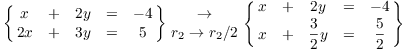
The row operation that adds a multiple of one row to another corresponds to adding a multiple of one equation to another. For example, I can add -2 times the first equation to the second equation (that is, subtract 2 times the first equation from the second equation):
![]()
You can see that row operations certainly correspond to "legal" operations that you can perform on systems of equations. You can even see in the last example how these operations might be used to solve a system.
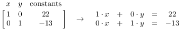
To make the connection with row reducing matrices, suppose we take our system and just write down the coefficients:
![]()
This matrix is called the augmented matrix or auxiliary matrix for the system.
Watch what happens when I row reduce the matrix to row-reduced echelon form!
![]()
Since row operations operate on rows, they will "preserve" the columns for the x-numbers, the y-numbers, and the constants: The coefficients of x in the equations will always be in the first column, regardless of what operations I perform, and so on for the y-coefficients and the constants. So at the end, I can put the variables back to get equations, reversing what I did at the start:
That is, ![]() and
and ![]() --- I solved the system!
--- I solved the system!
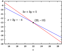
Geometrically, the graphs of ![]() and
and ![]() are lines. Solving simultaneously
amounts to finding where the lines intersect --- in this case, in the
point
are lines. Solving simultaneously
amounts to finding where the lines intersect --- in this case, in the
point ![]() .
.
(I will often write solutions to systems in the form ![]() , or even
, or even ![]() . In the second form, it's
understood that the variables occur in the same order in which they
occurred in the equations.)
. In the second form, it's
understood that the variables occur in the same order in which they
occurred in the equations.)
You can see several things from this example. First, we noted that row operations imitate the operations you might perform on whole equations to solve a system. This explains why row operations are what they are.
Second, you can see that having row reduced echelon form as the target of a row reduction corresponds to producing equations with "all the variables solved for". Think particularly of the requirements that leading entries (the 1's) must be the only nonzero elements in their columns, and the "stairstep" pattern of the leading entries.
Third, by working with the coefficients of the variables and the constants, we save ourselves the trouble of writing out the equations. We "get lazy" and only write exactly what we need to write to do the problem: The matrix preserves the structure of the equations for us. (This idea of "detaching coefficients" is useful in other areas of math.)
Let's see some additional examples.
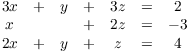
Example. Use row reduction to solve the
following system of linear equations over ![]() :
:
Write down the matrix for the system and row reduce it to row reduced echelon form:
![$$ \left[\matrix{ 1 & 1 & 1 & 5 \cr 1 & 3 & 1 & 9 \cr 4 & -1 & 1 & -2 \cr}\right] \matrix{\to \cr r_{3} \to r_{3} - 4 r_{1} \cr} \left[\matrix{ 1 & 1 & 1 & 5 \cr 1 & 3 & 1 & 9 \cr 0 & -5 & -3 & -22 \cr}\right] \matrix{\to \cr r_{2} \to r_{2} - r_{1} \cr} \left[\matrix{ 1 & 1 & 1 & 5 \cr 0 & 2 & 0 & 4 \cr 0 & -5 & -3 & -22 \cr}\right] \matrix{\to \cr r_{2} \to \dfrac{1}{2} r_{2} \cr}$$](solving-systems-of-linear-equations47.png)
![$$\left[\matrix{ 1 & 1 & 1 & 5 \cr 0 & 1 & 0 & 2 \cr 0 & -5 & -3 & -22 \cr}\right] \matrix{\to \cr r_{1} \to r_{1} - r_{2} \cr} \left[\matrix{ 1 & 0 & 1 & 3 \cr 0 & 1 & 0 & 2 \cr 0 & -5 & -3 & -22 \cr}\right] \matrix{\to \cr r_{3} \to r_{3} + 5 r_{2} \cr} \left[\matrix{ 1 & 0 & 1 & 3 \cr 0 & 1 & 0 & 2 \cr 0 & 0 & -3 & -12 \cr}\right] \matrix{\to \cr r_{3} \to -\dfrac{1}{3} r_{3} \cr}$$](solving-systems-of-linear-equations48.png)
![$$\left[\matrix{ 1 & 0 & 1 & 3 \cr 0 & 1 & 0 & 2 \cr 0 & 0 & 1 & 4 \cr}\right] \matrix{\to \cr r_{1} \to r_{1} - r_{3} \cr} \left[\matrix{ 1 & 0 & 0 & -1 \cr 0 & 1 & 0 & 2 \cr 0 & 0 & 1 & 4 \cr}\right]$$](solving-systems-of-linear-equations49.png)
The last matrix represents the equations ![]() ,
, ![]() ,
, ![]() . So the solution is
. So the solution is ![]() .
.![]()
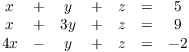
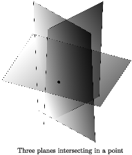
In this case, the three equations represent planes in space, and the
point ![]() is the intersection of the
three planes.
is the intersection of the
three planes.
Everything works in similar fashion for systems of linear equations
over a finite field. Here's an example over ![]() .
.
Example. Solve the following system of linear
equations over ![]() :
:
Remember that all the arithmetic is done in ![]() . So, for example,
. So, for example,
![]()
The last equation tells you that when you would think of dividing by 2, you multiply by 2 instead.
Write down the corresponding matrix and row reduce it to row reduced echelon form:
![$$\left[\matrix{ 1 & 2 & 0 & 2 \cr 2 & 1 & 1 & 1 \cr 2 & 0 & 1 & 2 \cr}\right] \matrix{\to \cr r_{3} \to r_{3} + r_{1} \cr} \left[\matrix{ 1 & 2 & 0 & 2 \cr 2 & 1 & 1 & 1 \cr 0 & 2 & 1 & 1 \cr}\right] \matrix{\to \cr r_{2} \to r_{2} + r_{1} \cr} \left[\matrix{ 1 & 2 & 0 & 2 \cr 0 & 0 & 1 & 0 \cr 0 & 2 & 1 & 1 \cr}\right] \matrix{\to \cr r_{2} \leftrightarrow r_{3} \cr}$$](solving-systems-of-linear-equations61.png)
![$$\left[\matrix{ 1 & 2 & 0 & 2 \cr 0 & 2 & 1 & 1 \cr 0 & 0 & 1 & 0 \cr}\right] \matrix{\to \cr r_{2} \to 2 r_{2} \cr} \left[\matrix{ 1 & 2 & 0 & 2 \cr 0 & 1 & 2 & 2 \cr 0 & 0 & 1 & 0 \cr}\right] \matrix{\to \cr r_{1} \to r_{1} + r_{2} \cr} \left[\matrix{ 1 & 0 & 2 & 1 \cr 0 & 1 & 2 & 2 \cr 0 & 0 & 1 & 0 \cr}\right] \matrix{\to \cr r_{1} \to r_{1} + r_{3} \cr}$$](solving-systems-of-linear-equations62.png)
![$$\left[\matrix{ 1 & 0 & 0 & 1 \cr 0 & 1 & 2 & 2 \cr 0 & 0 & 1 & 0 \cr}\right] \matrix{\to \cr r_{2} \to r_{2} + r_{3} \cr} \left[\matrix{ 1 & 0 & 0 & 1 \cr 0 & 1 & 0 & 2 \cr 0 & 0 & 1 & 0 \cr}\right]$$](solving-systems-of-linear-equations63.png)
The last matrix represents the equations ![]() ,
, ![]() ,
, ![]() . Hence, the solution is
. Hence, the solution is ![]() .
.![]()
It's possible for a system of linear equations to have no solutions.
Such a system is said to be inconsistent. You
can tell a system of linear equations is inconsistent if at any point
one of the equations gives a contradiction, such as "![]() " or "
" or "![]() ".
".
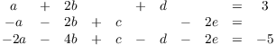
Example. Solve the following system of
equations over ![]() :
:
Form the coefficient matrix and row reduce:
![$$\left[\matrix{ 3 & 1 & 3 & 2 \cr 1 & 0 & 2 & -3 \cr 2 & 1 & 1 & 4 \cr}\right] \quad\to\quad \left[\matrix{ 1 & 0 & 2 & 0 \cr 0 & 1 & -3 & 0 \cr 0 & 0 & 0 & 1 \cr}\right]$$](solving-systems-of-linear-equations72.png)
The corresponding equations are
![]()
The last equation says ![]() . Hence, the system has no
solutions.
. Hence, the system has no
solutions.![]()
Note: If you're row reducing to solve a system and you notice that a
row of the current matrix would give an equation that is a
contradiction (like "![]() " or "
" or "![]() "), you can stop row reducing
and conclude that there is no solution; you don't need to go all the
way to row reduced echelon form.
"), you can stop row reducing
and conclude that there is no solution; you don't need to go all the
way to row reduced echelon form.
Besides a single solution or no solutions, a system of linear equations can have many solutions. When this happens, we'll express the solutions in parametrized or parametric form. Here's an example over the real numbers.
Example. Solve the following system of linear
equations over ![]() :
:
Write down the corresponding matrix and row reduce:
![$$\left[\matrix{ 1 & 2 & 0 & 1 & 0 & 3 \cr -1 & -2 & 1 & 0 & -2 & -2 \cr -2 & -4 & 1 & -1 & -2 & -5 \cr}\right] \matrix{\to \cr r_{3} \to r_{3} + 2 r_{1} \cr} \left[\matrix{ 1 & 2 & 0 & 1 & 0 & 3 \cr -1 & -2 & 1 & 0 & -2 & -2 \cr 0 & 0 & 1 & 1 & -2 & 1 \cr}\right] \matrix{\to \cr r_{2} \to r_{2} + r_{1} \cr}$$](solving-systems-of-linear-equations79.png)
![$$\left[\matrix{ 1 & 2 & 0 & 1 & 0 & 3 \cr 0 & 0 & 1 & 1 & -2 & 1 \cr 0 & 0 & 1 & 1 & -2 & 1 \cr}\right] \matrix{\to \cr r_{3} \to r_{3} - r_{2} \cr} \left[\matrix{ 1 & 2 & 0 & 1 & 0 & 3 \cr 0 & 0 & 1 & 1 & -2 & 1 \cr 0 & 0 & 0 & 0 & 0 & 0 \cr}\right]$$](solving-systems-of-linear-equations80.png)
The corresponding equations are
![]()
Notice that the variables are not solved for as particular numbers. This means that the system will have more than one solution. In this case, we'll write the solution in parametric form.
The variables a and c correspond to leading entries in the row reduced echelon matrix. b, d, and e are called free variables. Solve for the leading entry variables a and c in terms of the free variables b, d, and e:
![]()
Next, assign parameters to each of the free variables b, d, and e. Often variables like s, t, u, and v are used as parameters. Try to pick variables "on the other side of the alphabet" from the original variables to avoid confusion. I'll use
![]()
Plugging these into the equations for a and c gives
![]()
All together, the solution is
(I lined up the variables so you can see the structure of the solution. You don't need to do this in problems for now, but it will be useful when we discuss how to find the basis for the null space of a matrix.)
Each assignment of numbers to the parameters s, t, and u produces a
solution. For example, if ![]() ,
, ![]() , and
, and ![]() ,
,
![]()
The solution (in this case) is ![]() . Since you
can assign any real number to each of s, t, and u, there are
infinitely many solutions.
. Since you
can assign any real number to each of s, t, and u, there are
infinitely many solutions.
Geometrically, the 3 original equations represented sets in
5-dimensional space ![]() . The solution to the system
represents the intersection of those 3 sets. Since the
solution has 3 parameters, the intersection is some kind of
3-dimensional set. Since the sets are in 5-dimensional space, it
would not be easy to draw a picture!
. The solution to the system
represents the intersection of those 3 sets. Since the
solution has 3 parameters, the intersection is some kind of
3-dimensional set. Since the sets are in 5-dimensional space, it
would not be easy to draw a picture!![]()
Example. Solve the following system over ![]() :
:
Write down the matrix for the system and row reduce:
![$$\left[\matrix{1 & 1 & 1 & 2 & 1 \cr 0 & 2 & 2 & 1 & 0 \cr 2 & 0 & 2 & 1 & 1 \cr}\right] \matrix{\rightarrow \cr r_3\to r_3-2 r_1 \cr} \left[\matrix{1 & 1 & 1 & 2 & 1 \cr 0 & 2 & 2 & 1 & 0 \cr 0 & 3 & 0 & 2 & 4 \cr}\right] \matrix{\rightarrow \cr r_2\to 3 r_2 \cr} \left[\matrix{1 & 1 & 1 & 2 & 1 \cr 0 & 1 & 1 & 3 & 0 \cr 0 & 3 & 0 & 2 & 4 \cr}\right] \matrix{\rightarrow \cr r_1\to r_1-r_2 \cr}$$](solving-systems-of-linear-equations94.png)
![$$\left[\matrix{1 & 0 & 0 & 4 & 1 \cr 0 & 1 & 1 & 3 & 0 \cr 0 & 3 & 0 & 2 & 4 \cr}\right] \matrix{\rightarrow \cr r_3\to r_3-3 r_2 \cr} \left[\matrix{1 & 0 & 0 & 4 & 1 \cr 0 & 1 & 1 & 3 & 0 \cr 0 & 0 & 2 & 3 & 4 \cr}\right] \matrix{\rightarrow \cr r_3\to 3 r_3 \cr} \left[\matrix{1 & 0 & 0 & 4 & 1 \cr 0 & 1 & 1 & 3 & 0 \cr 0 & 0 & 1 & 4 & 2 \cr}\right] \matrix{\rightarrow \cr r_2\to r_2-r_3 \cr}$$](solving-systems-of-linear-equations95.png)
![$$\left[\matrix{1 & 0 & 0 & 4 & 1 \cr 0 & 1 & 0 & 4 & 3 \cr 0 & 0 & 1 & 4 & 2 \cr}\right]$$](solving-systems-of-linear-equations96.png)
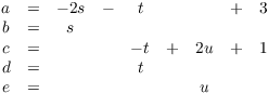
Putting the variables back, the corresponding equations are
![]()
Solve for the leading entry variables w, x, and y in terms of the
free variable z. Note that ![]() , so I can solve by adding z to
each of the 3 equations:
, so I can solve by adding z to
each of the 3 equations:
![]()
To write the solution in parametric form, assign a parameter to the
"non-leading entry" variable z. Thus, set ![]() :
:
![]()
Remember that the number system is ![]() . So there
are 5 possible values for the parameter t, and each value of t gives
a solution. For instance, if
. So there
are 5 possible values for the parameter t, and each value of t gives
a solution. For instance, if ![]() , I get
, I get
![]()
It follows that this system of equations has 5 solutions.![]()
Remark. A system of linear equations over the real numbers can have no solutions, a unique solution, or infinitely many solutions. (That is, such a system can't have exactly 3 solutions.)
On the other hand, if p is prime, a system of linear equations over
![]() will have
will have ![]() solutions, for
solutions, for ![]() , or no solutions. For example, a
system over
, or no solutions. For example, a
system over ![]() can have no
solutions, one (that is,
can have no
solutions, one (that is, ![]() ) solution, 5 solutions, 25 solutions, and
so on.
) solution, 5 solutions, 25 solutions, and
so on.
Remember that if A is a square (![]() ) matrix, the
inverse
) matrix, the
inverse ![]() of A is an
of A is an ![]() matrix such that
matrix such that
![]()
Here I is the ![]() identity
matrix. Note that not every square matrix has an inverse.
identity
matrix. Note that not every square matrix has an inverse.
Row reduction provides a systematic way to find the inverse of a matrix. The algorithm gives another application of row reduction, so I'll describe the algorithm and give an example. We'll justify the algorithm later.
To invert a matrix, adjoin a copy of the identity matrix to the original matrix. "Adjoin" means to place a copy of the identity matrix of the same size as the original matrix on the right of the original matrix to form a larger matrix (the augmented matrix).
Next, row reduce the augmented matrix. When the block corresponding the original matrix becomes the identity, the block corresponding to the identity will have become the inverse.
Example. Invert the following matrix over ![]() :
:
![]()
Place a copy of the ![]() identity matrix on the right of
the original matrix, then row reduce the augmented matrix:
identity matrix on the right of
the original matrix, then row reduce the augmented matrix:
![$$\left[\matrix{ 2 & -1 & 1 & 0 \cr 5 & -3 & 0 & 1 \cr}\right] \matrix{\to \cr r_{1} \to \dfrac{1}{2} r_{1} \cr} \left[\matrix{ 1 & -\dfrac{1}{2} & \dfrac{1}{2} & 0 \cr \noalign{\vskip2pt} 5 & -3 & 0 & 1 \cr}\right] \matrix{\to \cr r_{2} \to r_{2} - 5 r_{1} \cr} \left[\matrix{ 1 & -\dfrac{1}{2} & \dfrac{1}{2} & 0 \cr \noalign{\vskip2pt} 0 & -\dfrac{1}{2} & -\dfrac{5}{2} & 1 \cr}\right] \matrix{\to \cr r_{2} \to -2 r_{2} \cr}$$](solving-systems-of-linear-equations118.png)
![$$ \left[\matrix{ 1 & -\dfrac{1}{2} & \dfrac{1}{2} & 0 \cr \noalign{\vskip2pt} 0 & 1 & 5 & -2 \cr}\right] \matrix{\to \cr r_{1} \to r_{1} + \dfrac{1}{2} r_{2} \cr} \left[\matrix{ 1 & 0 & 3 & -1 \cr 0 & 1 & 5 & -2 \cr}\right]$$](solving-systems-of-linear-equations119.png)
You can see that the original matrix in the left-hand ![]() block has turned into the
block has turned into the ![]() identity matrix. The identity
matrix that was in the right-hand
identity matrix. The identity
matrix that was in the right-hand ![]() block has at the same time turned
into the inverse.
block has at the same time turned
into the inverse.
Therefore, the inverse is
![]()
You can check that
![]()
Of course, there's a formula for inverting a ![]() matrix. But the procedure above
works with (square) matrices of any size. To explain why
this algorithm works, I'll need to examine the relationship between
row operations and inverses more closely.
matrix. But the procedure above
works with (square) matrices of any size. To explain why
this algorithm works, I'll need to examine the relationship between
row operations and inverses more closely.
You might have discussed lines and planes in 3 dimensions in a calculus course; if so, you probably saw problems like the next example. The rule of thumb is: You can often find the intersection of things by solving equations simultaneously.
Example. Find the line of intersection of the
planes in ![]() :
:
![]()
Think of the equations as a system of linear equations over ![]() . Write down the coefficient
matrix and row reduce:
. Write down the coefficient
matrix and row reduce:
![]()
![$$\left[\matrix{ 1 & 2 & -1 & 4 \cr \noalign{\vskip2pt} 0 & 1 & 0 & \dfrac{1}{3} \cr}\right] \matrix{\to \cr r_{1} \to r_{1} - 2 r_{2} \cr} \left[\matrix{ 1 & 0 & -1 & \dfrac{10}{3} \cr \noalign{\vskip2pt} 0 & 1 & 0 & \dfrac{1}{3} \cr}\right]$$](solving-systems-of-linear-equations130.png)
The last matrix gives the equations
![]()
Thus, ![]() and
and ![]() . Letting
. Letting ![]() , the parametric solution is
, the parametric solution is
![]()
These are the parametric equations of the line of intersection.![]()
The solution of simultaneous linear equations dates back 2000 years to the Jiuzhang Suanshu, a collection of problems compiled in China. The systematic algebraic process of eliminating variables seems to be due to Isaac Newton. Matrix notation developed in the second half of the 1800's; what we call Gaussian elimination, applied to matrices, was developed in the first half of the 1900's by various mathematicians. Grcar [1] contains a nice historical account.
[1] Joseph Grcar, Mathematics of Gaussian elimination, Notices of the American Mathematical Society, 58(6)(2011), 782--792.
Copyright 2021 by Bruce Ikenaga