Vector spaces and linear transformations are the primary objects of study in linear algebra. A vector space (which I'll define below) consists of two sets: A set of objects called vectors and a field (the scalars).
You may have seen vectors before --- in physics or engineering courses, or in multivariable calculus. In those courses, you tend to see particular kinds of vectors, and it could lead you to think that those particular kinds of vectors are the only kinds of vectors. We'll discuss vectors by giving axioms for vectors. When you define a mathematical object using a set of axioms, you are describing how it behaves. Why is this important?
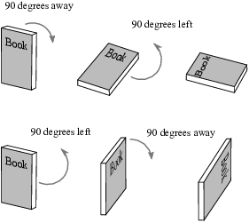
One common intuitive description of vectors is that they're things which "have a magnitude and a direction". This isn't a bad description for certain kinds of vectors, but it has some shortcomings. Consider the following example: Take a book and hold it out in front of you with the cover facing toward you.
First, rotate the book ![]() away from you,
then (without returning the book to its original position) rotate the
book
away from you,
then (without returning the book to its original position) rotate the
book ![]() to your left. The first three pictures
illustrate the result.
to your left. The first three pictures
illustrate the result.
Next, return the book to its original position facing you. Rotate the
book ![]() to your left, then (without returning the
book to its original position) rotate the book (without returning the
book to its original position) away from you. The next three pictures
illustrate the result.
to your left, then (without returning the
book to its original position) rotate the book (without returning the
book to its original position) away from you. The next three pictures
illustrate the result.
In other words, we're doing two rotations --- ![]() away from you and
away from you and ![]() to your left
--- one after the other, in the two possible orders. Note that the
final positions are different.
to your left
--- one after the other, in the two possible orders. Note that the
final positions are different.
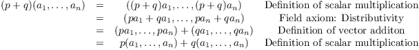
It's certainly reasonable to say that rotations by ![]() away from you or to your left are things with
"magnitudes" and "directions". And it seems
reasonable to "add" such rotations by doing one followed by
the other. However, we saw that when we performed the
"addition" in different orders, we got different results.
Symbolically,
away from you or to your left are things with
"magnitudes" and "directions". And it seems
reasonable to "add" such rotations by doing one followed by
the other. However, we saw that when we performed the
"addition" in different orders, we got different results.
Symbolically,
![]()
The addition fails to be commutative. But it happens that we really do want vector addition to be commutative, for all of the "vectors" that come up in practice.
It is not enough to tell what a thing "looks like" ("magnitude and direction"); we need to say how the thing behaves. This example also showed that words like "magnitude" and "direction" are ambiguous.
Other descriptions of vectors --- as "arrow", or as "lists of numbers" --- also describe particular kinds of vectors. And as with "magnitude and direction", they're incomplete: They don't tell how the "vectors" in question behave.
Our axioms for a vector space describe how vectors should behave --- and if they behave right, we don't care what they look like! It's okay to think of "magnitude and direction" or "arrow" or "list of numbers", as long as you remember that these are only particular kinds of vectors.
Let's see the axioms for a vector space.
Definition. A vector
space V over a field F is a set V equipped with two operations.
The first is called (vector) addition; it
takes vectors u and v and produces another vector ![]() .
.
The second operation is called scalar
multiplication; it takes an element ![]() and a vector
and a vector ![]() and produces a vector
and produces a vector ![]() .
.
These operations satisfy the following axioms:
1. Vector addition is associative: If ![]() , then
, then
![]()
2. Vector addition is commutative: If ![]() , then
, then
![]()
3. There is a zero vector 0 which satisfies
![]()
Note: Some people prefer to write something like "![]() " for the zero vector to distinguish it from the
number 0 in the field F. I'll be a little lazy and just write
"0" and rely on you to determine whether it's the zero
vector or the number zero from the context.
" for the zero vector to distinguish it from the
number 0 in the field F. I'll be a little lazy and just write
"0" and rely on you to determine whether it's the zero
vector or the number zero from the context.
4. For every vector ![]() , there is a vector
, there is a vector ![]() which satisfies
which satisfies
![]()
5. If ![]() and
and ![]() , then
, then
![]()
6. If ![]() and
and ![]() , then
, then
![]()
7. If ![]() and
and ![]() , then
, then
![]()
8. If ![]() , then
, then
![]()
The elements of V are called vectors; the elements of F are called scalars. As usual, the use of words like "multiplication" does not imply that the operations involved look like ordinary "multiplication".
Note that Axiom (4) allows us to define subtraction of vectors this way:
![]()
An easy (and trivial) vector space (over any field F) is the zero vector space ![]() . It consists of
a zero vector (which is required by Axiom 3) and nothing else. The
scalar multiplication is
. It consists of
a zero vector (which is required by Axiom 3) and nothing else. The
scalar multiplication is ![]() for any
for any ![]() . You can easily check that all the axioms hold.
. You can easily check that all the axioms hold.
The most important example of a vector space over a field F is given
by the "standard" vector space ![]() . In fact, every (finite-dimensional) vector space
over F is isomorphic to
. In fact, every (finite-dimensional) vector space
over F is isomorphic to ![]() for some nonnegative integer n. We'll discuss
isomorphisms later; let's give the definition of
for some nonnegative integer n. We'll discuss
isomorphisms later; let's give the definition of ![]() .
.
If F is a field and ![]() , then
, then ![]() denotes the set
denotes the set
![]()
If you know about (Cartesian) products, you can see that ![]() is the product of n copies of F.
is the product of n copies of F.
We can also define ![]() to be the zero vector space
to be the zero vector space ![]() .
.
If ![]() and
and ![]() , I'll
often refer to
, I'll
often refer to ![]() ,
, ![]() , ...
, ... ![]() as the components of v.
as the components of v.
Proposition. ![]() becomes a vector space
over F with the following operations:
becomes a vector space
over F with the following operations:
![]()
![]()
![]() is called the vector space of
n-dimensional vectors over F. The elements
is called the vector space of
n-dimensional vectors over F. The elements ![]() , ...,
, ..., ![]() are called the vector's components.
are called the vector's components.
Proof. I'll check a few of the axioms by way of example.
To check Axiom 2, take ![]() and write
and write
![]()
Thus, ![]() for
for ![]() .
.
Then
![]()
![]()
The second equality used the fact that ![]() for
each i, because the u's and v's are elements of the field F, and
addition in F is commutative.
for
each i, because the u's and v's are elements of the field F, and
addition in F is commutative.
The zero vector is ![]() (n components). I'll
use "0" to denote the zero vector as well as the number 0
in the field F; the context should make it clear which of the two is
intended. For instance, if v is a vector and I write "
(n components). I'll
use "0" to denote the zero vector as well as the number 0
in the field F; the context should make it clear which of the two is
intended. For instance, if v is a vector and I write "![]() ", the "0" must be the zero vector,
since adding the number 0 to the vector v is not defined.
", the "0" must be the zero vector,
since adding the number 0 to the vector v is not defined.
If ![]() , then
, then
![]()
Since I already showed that addition of vectors is commutative, it
follows that ![]() as well. This verifies Axiom 3.
as well. This verifies Axiom 3.
If ![]() , then I'll define
, then I'll define ![]() . Then
. Then
![]()
Commutativity of addition gives ![]() as well, and
this verifies Axiom 4.
as well, and
this verifies Axiom 4.
I'll write out the proof Axiom 6 in a little more detail. Let ![]() , and let
, and let ![]() . Then
. Then
You can see that checking the axioms amounts to writing out the
vectors in component form, applying the definitions of vector
addition and scalar multiplication, and using the axioms for a
field.![]()
While all vector spaces "look like" ![]() (at least if "n" is allowed to be infinite
--- the fancy word is "isomorphism"), you should not assume
that a given vector space is
(at least if "n" is allowed to be infinite
--- the fancy word is "isomorphism"), you should not assume
that a given vector space is ![]() , unless you're
explicitly told that it is. We'll see examples (like
, unless you're
explicitly told that it is. We'll see examples (like ![]() below) where it's not easy to see why a given vector
space "looks like"
below) where it's not easy to see why a given vector
space "looks like" ![]() .
.
In discussing matrices, we've referred to a matrix with a single row as a row vector and a matrix with a single column as a column vector.
![$$\matrix{ \left[\matrix{1 & 2 & 3 \cr}\right] & \left[\matrix{1 \cr 2 \cr 3 \cr}\right] \cr \noalign{\vskip2pt} \hbox{row vector} & \hbox{column vector} \cr}$$](vector-spaces80.png)
The elements of ![]() are just ordered n-tuples, not matrices. In
certain situations, we may "identify" a vector in
are just ordered n-tuples, not matrices. In
certain situations, we may "identify" a vector in ![]() with a row vector or a column vector in the obvious
way:
with a row vector or a column vector in the obvious
way:
![$$(1, 2, 3) \leftrightarrow \left[\matrix{1 & 2 & 3 \cr}\right] \leftrightarrow \left[\matrix{1 \cr 2 \cr 3 \cr}\right]$$](vector-spaces83.png)
(Very often, we'll use a column vector, for reasons we'll see later.)
I will mention this identification explicitly if we're doing this,
but for right now just think of ![]() as an ordered
triple, not a matrix.
as an ordered
triple, not a matrix.
You may have seen examples of ![]() -vector spaces before.
-vector spaces before.
For instance, ![]() consists of 3-dimensional vectors with real
components, like
consists of 3-dimensional vectors with real
components, like
![]()
You're probably familiar with addition and scalar multiplication for these vectors:
![]()
![]()
Note: Some people write ![]() as "
as "![]() ", using angle brackets to distinguish
vectors from points.
", using angle brackets to distinguish
vectors from points.
Recall that ![]() is the field
is the field ![]() , where the operations are addition and
multiplication mod 3. Thus,
, where the operations are addition and
multiplication mod 3. Thus, ![]() consists of
2-dimensional vectors with components in
consists of
2-dimensional vectors with components in ![]() . Since each of the two components can be any element
in
. Since each of the two components can be any element
in ![]() , there are
, there are ![]() such
vectors:
such
vectors:
![]()
Here are examples of vector addition and multiplication in ![]() :
:
![]()
![]()
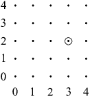
We can picture elements of ![]() as points in
n-dimensional space. Let's look at
as points in
n-dimensional space. Let's look at ![]() , since it's easy
to draw the pictures.
, since it's easy
to draw the pictures. ![]() is the x-y-plane, and elements of
is the x-y-plane, and elements of
![]() are points in the plane:
are points in the plane:
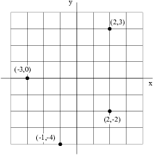
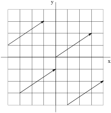
In the picture above, each grid square is ![]() . The vectors
. The vectors ![]() ,
, ![]() ,
, ![]() , and
, and ![]() are shown.
are shown.
Vectors in ![]() are often drawn as arrows going from the
origin
are often drawn as arrows going from the
origin ![]() to the corresponding point. Here's
how the vectors in the previous picture look when represented with
arrows:
to the corresponding point. Here's
how the vectors in the previous picture look when represented with
arrows:
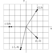
If the x-component is negative, the arrow goes to the left; if the y-component is negative, the arrow goes down.
When you represent vectors in ![]() as arrows, the
arrows do not have to start at the origin. For instance, in
as arrows, the
arrows do not have to start at the origin. For instance, in ![]() the vector
the vector ![]() can be represented by any
arrow which goes 3 units in the x-direction and 2 units in the
y-direction, from the start of the arrow to the end of the arrow. All
of the arrows in the picture below represent the vector
can be represented by any
arrow which goes 3 units in the x-direction and 2 units in the
y-direction, from the start of the arrow to the end of the arrow. All
of the arrows in the picture below represent the vector ![]() :
:
As long as the length and direction of the arrow don't change as it is moved around, it represents the same vector.
Representing vectors in ![]() as arrows gives us
a way of picturing vector addition, vector subtraction, and scalar
multiplication.
as arrows gives us
a way of picturing vector addition, vector subtraction, and scalar
multiplication.
To add vectors a and b represented as arrows, move one of the arrows --- say b --- so that it starts at the end of the vector a. As you move b, keep its length and direction the same:
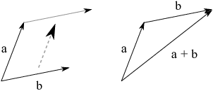
As we noted earlier, if you don't change an arrow's length or
direction, it represents the same vector. So the new vector is still
b. The sum ![]() is represented by the arrow that goes from
the start of a to the end of b.
is represented by the arrow that goes from
the start of a to the end of b.
You can also leave b alone and move a so it starts at the end of b.
Then ![]() is the arrow going from the start of b to the end of
a. Notice that it's the same as the arrow
is the arrow going from the start of b to the end of
a. Notice that it's the same as the arrow ![]() , which reflects the commutativity of vector
addition:
, which reflects the commutativity of vector
addition: ![]() .
.
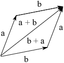
This picture also shows that you can think of ![]() (or
(or ![]() ) as the arrow given by the
diagonal of the parallelogram whose sides are a and b.
) as the arrow given by the
diagonal of the parallelogram whose sides are a and b.
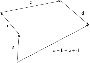
You can add more than two vectors in the same way. Move the vectors to make a chain, so that the next vector's arrow starts at the end of the previous vector's arrow. The sum is the arrow that goes from the start of the first arrow to the end of the last arrow:
To subtract a vector b from a vector a --- that is, to do ![]() --- draw the arrow from the end of b to the end of a.
This assumes that the arrows for a and b start at the same point:
--- draw the arrow from the end of b to the end of a.
This assumes that the arrows for a and b start at the same point:
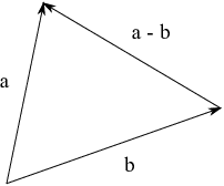
To see that this picture is correct, interpret it as an addition
picture, where we're adding ![]() to b. The sum
to b. The sum ![]() should be the arrow from the start of b to
the end of
should be the arrow from the start of b to
the end of ![]() , which it is.
, which it is.
When a vector a is multiplied by a real number k to get ![]() , the arrow representing the vector is scaled up by a
factor of k. In addition, if k is negative, the arrow is
"flipped"
, the arrow representing the vector is scaled up by a
factor of k. In addition, if k is negative, the arrow is
"flipped" ![]() , so it points in the opposite
direction to the arrow for a.
, so it points in the opposite
direction to the arrow for a.
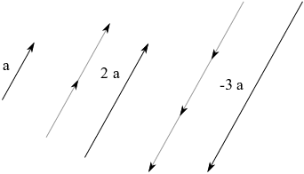
In the picture above, the vector ![]() is twice as long as a
and points in the same direction as a. The vector
is twice as long as a
and points in the same direction as a. The vector ![]() is 3 times as long as a, but points in the opposite
direction.
is 3 times as long as a, but points in the opposite
direction.
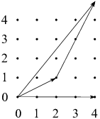
Example. Three vectors in ![]() are shown in the picture below.
are shown in the picture below.
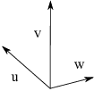
Draw the vector ![]() .
.
I start by constructing ![]() , an arrow twice as long as v in
the same direction as v. I place it so it starts at the same place as
u. Then the arrow that goes from the end of
, an arrow twice as long as v in
the same direction as v. I place it so it starts at the same place as
u. Then the arrow that goes from the end of ![]() to the end of u is
to the end of u is ![]() .
.
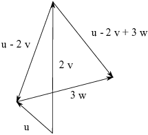
Next, I construct ![]() , an arrow 3 times as long as w in
the same direction as w. I move
, an arrow 3 times as long as w in
the same direction as w. I move ![]() so it starts at the
end of
so it starts at the
end of ![]() . Then the arrow from the start of
. Then the arrow from the start of ![]() to the end of
to the end of ![]() is
is ![]() .
.![]()
While we can draw pictures of vectors when the field of scalars is
the real numbers ![]() , pictures don't work quite as
well with other fields. As an example, suppose the field is
, pictures don't work quite as
well with other fields. As an example, suppose the field is ![]() . Remember that the operations in
. Remember that the operations in
![]() are addition mod 5 and multiplication mod 5. So, for
instance,
are addition mod 5 and multiplication mod 5. So, for
instance,
![]()
We saw that ![]() is just the x-y plane. What about
is just the x-y plane. What about ![]() ? It consists of pairs
? It consists of pairs ![]() where a and b are elements of
where a and b are elements of ![]() . Since there are 5 choices for a and 5 choices for
b, there are
. Since there are 5 choices for a and 5 choices for
b, there are ![]() elements in
elements in ![]() . We can picture it as a
. We can picture it as a ![]() grid of dots:
grid of dots:
The dot corresponding to the vector ![]() is circled as an
example.
is circled as an
example.
Picturing vectors as arrows seems to work until we try to do vector
arithmetic. For example, suppose ![]() in
in ![]() . We can represent it with an arrow from the origin
to the point
. We can represent it with an arrow from the origin
to the point ![]() .
.
Suppose we multiply v by 2. You can check that ![]() .
.
Here's a picture showing ![]() and
and ![]() :
:
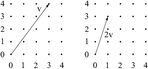
In ![]() , we'd expect
, we'd expect ![]() to have the same direction as
v and twice the length. You can see that it doesn't work that way in
to have the same direction as
v and twice the length. You can see that it doesn't work that way in
![]() .
.
What about vector addition in ![]() ? Suppose we
add
? Suppose we
add ![]() and
and ![]() :
:
![]()
If we represent the vectors as arrows and try to add the arrows as we
did in ![]() , we encounter problems. First, when I move
, we encounter problems. First, when I move
![]() so that it starts at the end of
so that it starts at the end of ![]() , the end of
, the end of ![]() sticks outside of
the
sticks outside of
the ![]() grid which represents
grid which represents ![]() .
.
If I ignore this problem and I draw the arrow from the start of ![]() to the end of
to the end of ![]() , the diagonal
arrow which should represent the sum looks very different from the
actual sum arrow
, the diagonal
arrow which should represent the sum looks very different from the
actual sum arrow ![]() (the horizontal arrow in the
picture) --- and as with
(the horizontal arrow in the
picture) --- and as with ![]() , the end of the sum arrow
sticks outside the grid which represents
, the end of the sum arrow
sticks outside the grid which represents ![]() .
.
You can see that thinking of vectors as arrows has limitations. It's
okay for vectors in ![]() .
.
What about thinking of vectors as "lists of numbers"? That
seemed to work in the examples above in ![]() and in
and in ![]() . In general,
this works for the
. In general,
this works for the ![]() vector spaces for finite n, but
those aren't the only vector spaces.
vector spaces for finite n, but
those aren't the only vector spaces.
Here are some examples of vector spaces which are not ![]() 's, at least for finite n.
's, at least for finite n.
The set ![]() of polynomials with real coefficients is a
vector space over
of polynomials with real coefficients is a
vector space over ![]() , using the standard operations on
polynomials. For example, you add polynomials and multiply them by
numbers in the usual ways:
, using the standard operations on
polynomials. For example, you add polynomials and multiply them by
numbers in the usual ways:
![]()
![]()
Unlike ![]() , the set of polynomials
, the set of polynomials ![]() is infinite dimensional.
(We'll discuss the dimension of a vector space
more precisely later). Intuitively, you need an infinite set of
polynomials, like
is infinite dimensional.
(We'll discuss the dimension of a vector space
more precisely later). Intuitively, you need an infinite set of
polynomials, like ![]() to
"construct" all the elements of
to
"construct" all the elements of ![]() .
.
You might notice that we can represent polynomials as "lists of numbers", as long as we're willing to allow infinite lists. For example,
![]()
We have to begin with the lowest degree coefficient and work our way
up, because polynomials can have arbitrarily large degree. So a
polynomial whose highest power term was ![]() might have nonzero numbers from the zeroth slot up to
the "3" in the
might have nonzero numbers from the zeroth slot up to
the "3" in the ![]() slot,
followed by an infinite number of zeros.
slot,
followed by an infinite number of zeros.
Not bad! It's hard to see how we could think of these as "arrows", but at least we have something like our earlier examples.
However, sometimes you can't represent an element of a vector space as a "list of numbers", even if you allow an "infinite list".
Let ![]() denote the continuous real-valued functions
defined on the interval
denote the continuous real-valued functions
defined on the interval ![]() . You add functions
pointwise:
. You add functions
pointwise:
![]()
From calculus, you know that the sum of continuous functions is a
continuous function. For instance, if ![]() and
and ![]() , then
, then
![]()
If ![]() and
and ![]() , define scalar
multiplication in pointwise fashion:
, define scalar
multiplication in pointwise fashion:
![]()
For example, if ![]() and
and ![]() , then
, then
![]()
These operations make ![]() into an
into an ![]() -vector space.
-vector space.
![]() is infinite dimensional just like
is infinite dimensional just like ![]() . However, its dimension is
uncountably infinite, while
. However, its dimension is
uncountably infinite, while ![]() has countably infinite dimension over
has countably infinite dimension over ![]() . We can't represent elements of
. We can't represent elements of ![]() as a "list of numbers", even infinite lists
of numbers.
as a "list of numbers", even infinite lists
of numbers.
Thinking of vectors as arrows or lists of numbers is fine where it's appropriate. But be aware that those ways of thinking about vectors don't apply in every case.
Having seen some examples, let's wind up by proving some easy properties of vectors in vector spaces. The next result says that many of the "obvious" things you'd assume about vector arithmetic are true.
Proposition. Let V be a vector space over a field F.
(a) ![]() for all
for all ![]() .
.
Note: The "0" on the left is the number 0 in the field F, while the "0" on the right is the zero vector in V.
(b) ![]() for all
for all ![]() .
.
Note: On both the left and right, "0" denotes the zero vector in V.
(c) ![]() for all
for all ![]() .
.
(d) ![]() for all
for all ![]() .
.
Proof. (a) As I noted above, the "0"
on the left is the zero in F, whereas the "0" on the right
is the zero vector in V. We use a little trick, writing 0 as ![]() :
:
![]()
The first step used the definition of the number zero: "Zero plus anything gives the anything", so take the "anything" to be the number 0 itself. The second step used distributivity.
Next, I'll subtract ![]() from both sides. Just this once,
I'll show all the steps using the axioms. Start with the equation
above, and add
from both sides. Just this once,
I'll show all the steps using the axioms. Start with the equation
above, and add ![]() to both sides:
to both sides:
![$$\matrix{ 0 \cdot x = 0 \cdot x + 0 \cdot x & \cr 0 \cdot x + [-(0 \cdot x)] = (0 \cdot x + 0 \cdot x) + [-(0 \cdot x)] & \cr 0 = (0 \cdot x + 0 \cdot x) + [-(0 \cdot x)] & (\hbox{Axiom (4)}) \cr 0 = 0 \cdot x + (0 \cdot x + [-(0 \cdot x)]) & (\hbox{Axiom (1)}) \cr 0 = 0 \cdot x + 0 & (\hbox{Axiom (4)}) \cr 0 = 0 \cdot x & (\hbox{Axiom (3)}) \cr}$$](vector-spaces239.png)
Normally, I would just say: "Subtracting ![]() from both sides, I get
from both sides, I get ![]() ." It's important to go through a few simple
proofs based on axioms to ensure that you really can do them. But the
result isn't very surprising: You'd expect "zero times anything
to equal zero". In the future, I won't usually do elementary
proofs like this one in such detail.
." It's important to go through a few simple
proofs based on axioms to ensure that you really can do them. But the
result isn't very surprising: You'd expect "zero times anything
to equal zero". In the future, I won't usually do elementary
proofs like this one in such detail.
(b) Note that "0" on both the left and right denotes the zero vector, not the number 0 in F. I use the same idea as in the proof of (a):
![]()
The first step used the definition of the zero vector, and the second
used distributivity. Now subtract ![]() from both sides
to get
from both sides
to get ![]() .
.
(c) (The "-1" on the left is the scalar -1; the "![]() " on the right is the "negative" of
" on the right is the "negative" of
![]() .)
.)
![]()
(d)
![]()
Copyright 2022 by Bruce Ikenaga